# Required packages
# !pip install torch torchvision numpy plotly dash dash-bootstrap-components scikit-learn scikit-imageAppendix B — Perturbation-based XAI methods
This notebook is part of the MINERVA best-practice guides and is released under the Apache License, Version 2.0. The accompanying written guide is released under CC BY 4.0.
# ============================================
# Imports
# ============================================

from math import comb

import dash
import dash_bootstrap_components as dbc
import numpy as np
import plotly.graph_objects as go
import plotly.io as pio
import torch
import torch.nn as nn
import torch.nn.functional as F
import torchvision
import torchvision.transforms as transforms
from dash import Input, Output, State, dcc, html
from IPython.display import display
from plotly.subplots import make_subplots
from skimage.segmentation import slic
from sklearn.datasets import fetch_california_housing
from sklearn.linear_model import Ridge
from sklearn.model_selection import train_test_split
from sklearn.preprocessing import StandardScaler

torch.manual_seed(0)
np.random.seed(0)

pio.renderers.default = "notebook_connected"
import plotly.io as pio  # noqa: E402

pio.renderers.default = "plotly_mimetype"
B.1 Part 1 - Tabular setting: California Housing
In perturbation-based methods, some concepts are easier to illustrate and therefore easier to understand using tabular examples rather than vision examples. Working with such data will help us build intuition for the methods: PFI, ICE/PDP, LIME and KernelSHAP.
To illustrate these ideas, we will use the California Housing dataset as a running example.
This dataset aims to predict median house prices based on 8 features: MedInc, HouseAge, AveRooms, AveBedrms, Population, AveOccup, Latitude, Longitude.
# ============================================
# Data fetching
# ============================================

housing     = fetch_california_housing()
FEATURE_NAMES = list(housing.feature_names)
X_raw, y_raw  = housing.data.astype(np.float32), housing.target.astype(np.float32)

scaler      = StandardScaler()
X_scaled    = scaler.fit_transform(X_raw).astype(np.float32)

X_tr, X_te, y_tr, y_te = train_test_split(
    X_scaled, y_raw, test_size=0.2, random_state=0
)

X_tr_t = torch.tensor(X_tr)
y_tr_t = torch.tensor(y_tr)
X_te_t = torch.tensor(X_te)
y_te_t = torch.tensor(y_te)

print(f'Train set: {X_tr.shape}  |  Test set: {X_te.shape}')
print(f'Features: {FEATURE_NAMES}')
Train set: (16512, 8) | Test set: (4128, 8)
Features: ['MedInc', 'HouseAge', 'AveRooms', 'AveBedrms', 'Population', 'AveOccup', 'Latitude', 'Longitude']# ============================================
# Definition of the model for the tabular part
# ============================================
class TabularMLP(nn.Module):
"""Small MLP for regression on tabular data."""
def __init__(self, n_features: int):
super().__init__()
self.net = nn.Sequential(
nn.Linear(n_features, 64), nn.ReLU(),
nn.Linear(64, 64), nn.ReLU(),
nn.Linear(64, 32), nn.ReLU(),
nn.Linear(32, 1),
)
def forward(self, x):
return self.net(x).squeeze(-1)
def train_tabular(model, X, y, epochs=40, batch_size=256, lr=1e-3):
opt = torch.optim.Adam(model.parameters(), lr=lr)
crit = nn.MSELoss()
print('Training tabular MLP...')
for epoch in range(epochs):
perm = torch.randperm(X.size(0))
total = 0.0
for i in range(0, X.size(0), batch_size):
idx = perm[i:i+batch_size]
opt.zero_grad()
loss = crit(model(X[idx]), y[idx])
loss.backward()
opt.step()
total += loss.item()
if (epoch + 1) % 10 == 0:
with torch.no_grad():
val_rmse = crit(model(X_te_t), y_te_t).sqrt().item()
print(f' Epoch {epoch+1}/{epochs} val RMSE: {val_rmse:.4f}')
print('Done.')
return model
tab_model = TabularMLP(n_features=len(FEATURE_NAMES))
tab_model = train_tabular(tab_model, X_tr_t, y_tr_t)
tab_model.eval()
def predict_tabular(X_np: np.ndarray) -> np.ndarray:
"""Black-box predict: (N, 8) float32 → (N,) predictions."""
with torch.no_grad():
return tab_model(torch.tensor(X_np)).numpy()Training tabular MLP...
Epoch 10/40 val RMSE: 0.5853
Epoch 20/40 val RMSE: 0.5472
Epoch 30/40 val RMSE: 0.5389
Epoch 40/40 val RMSE: 0.5328
Done.B.1.1 1. Permutation Feature Importance (PFI)
Idea: if shuffling feature \(j\) across the dataset increases the error, then \(j\) is important.
Algorithm: 1. Measure baseline RMSE \(m_0\) on the test set
2. For each feature \(j\) and each of \(R\) repetitions: permute column \(j\), measure permuted RMSE \(m^{(r)}_{\pi_j}\)
3. \(\mathrm{PFI}(j) = \dfrac{1}{R}\displaystyle\sum_{r=1}^{R} \bigl(m^{(r)}_{\pi_j} - m_0\bigr)\)
On tabular data the result is immediately readable: “shuffling MedInc increases RMSE by 0.6” is a concrete, meaningful statement.
PFI is a global measure: it summarises importance across all samples, not for a single prediction.
def compute_pfi(X: np.ndarray, y: np.ndarray,
                predict_fn, n_repeats: int = 5) -> dict:
    """
    Returns dict with:
        importances_mean: (n_features,)  mean importance over repeats
        importances_std:  (n_features,)  std over repeats
        baseline_rmse:    scalar
    """
    baseline_mse  = np.mean((predict_fn(X) - y) ** 2)
    baseline_rmse = np.sqrt(baseline_mse)

    n_features    = X.shape[1]
    all_drops     = np.zeros((n_repeats, n_features))

    for rep in range(n_repeats):
        for j in range(n_features):
            X_perm       = X.copy()
            X_perm[:, j] = np.random.permutation(X_perm[:, j])
            rmse_perm    = np.sqrt(np.mean((predict_fn(X_perm) - y) ** 2))
            all_drops[rep, j] = rmse_perm - baseline_rmse   # positive = important

    return {
        'importances_mean': all_drops.mean(axis=0),
        'importances_std':  all_drops.std(axis=0),
        'baseline_rmse':    baseline_rmse,
    }
B.1.2 2.Individual Conditional Expectation (ICE) & Partial Dependence Plot (PDP)
Idea: sweep one feature across its full value range while holding all other features fixed at their observed values.
- ICE: one curve per sample — how does this specific prediction change as feature \(j\) varies?
- PDP: the average ICE curve — the marginal effect of feature \(j\) across the whole dataset
On tabular data the x-axis is genuine: MedInc going from 0.5 to 15, HouseAge from 1 to 52.
The shape of the PDP curve (linear, saturating, non-monotone) tells you how the model uses each feature.
ICE and PDP are complementary: if ICE curves all have the same shape, the PDP tells the full story. If ICE curves cross or diverge, the PDP average is misleading, then there are interaction effects.
def compute_ice_pdp(X: np.ndarray, feature_idx: int,
                    predict_fn, n_samples: int = 200,
                    n_grid: int = 40) -> dict:
    """
    Returns:
        grid:          (n_grid,)          feature values swept
        grid_original: (n_grid,)          back-transformed to original scale
        ice:           (n_samples, n_grid) per-sample prediction curves
        pdp:           (n_grid,)           mean curve
    """
    X_sub  = X[:n_samples].copy()
    f_min  = X_sub[:, feature_idx].min()
    f_max  = X_sub[:, feature_idx].max()
    grid   = np.linspace(f_min, f_max, n_grid).astype(np.float32)

    mean_  = scaler.mean_[feature_idx]
    std_   = scaler.scale_[feature_idx]
    grid_original = grid * std_ + mean_

    ice = np.zeros((n_samples, n_grid), dtype=np.float32)
    for g_idx, val in enumerate(grid):
        X_sweep = X_sub.copy()
        X_sweep[:, feature_idx] = val
        ice[:, g_idx] = predict_fn(X_sweep)

    return {
        'grid':           grid,
        'grid_original':  grid_original,
        'ice':            ice,
        'pdp':            ice.mean(axis=0),
    }
B.1.3 3. Local Interpretable Model-Agnostic Explanations (LIME) for tabular data
Idea: fit a simple (linear) model in the neighbourhood of a single instance to approximate the black box locally.
Algorithm (for tabular data): 1. Take instance \(x\) to explain
2. Sample \(N\) perturbed instances by adding Gaussian noise to each feature
3. Weight each sample by its proximity to \(x\) using a Gaussian kernel on distance. 4. Fit a weighted Ridge regression: perturbed features → black-box predictions
5. Regression coefficients = LIME attributions
On tabular data the coefficients are directly readable:
“MedInc +0.42 → prediction increases by 0.42 units” is a concrete local statement.
LIME attributions are local: they describe this specific prediction, not the model globally.
def compute_lime_tabular(x: np.ndarray, X_bg: np.ndarray,
                          predict_fn,
                          n_samples: int = 1000,
                          kernel_width: float = 0.75) -> np.ndarray:
    """
    LIME attribution for a single tabular instance `x` (shape: n_features,).

    Perturbations are drawn from N(x, sigma) where sigma is estimated
    from the background dataset column-wise std.

    Returns attribution vector of shape (n_features,).
    """
    n_features = x.shape[0]
    sigma      = X_bg.std(axis=0) + 1e-8

    # Sample perturbed instances around x
    noise      = np.random.randn(n_samples, n_features).astype(np.float32)
    X_perturb  = x[np.newaxis] + noise * sigma[np.newaxis]  # (N, F)

    # Black-box predictions
    preds      = predict_fn(X_perturb)   # (N,)

    # Proximity weights: Gaussian kernel on L2 distance (in normalised space)
    dists      = np.linalg.norm(noise, axis=1)              # (N,)
    weights    = np.exp(-(dists ** 2) / (2 * kernel_width ** 2))

    # Weighted Ridge regression
    ridge      = Ridge(alpha=0.01, fit_intercept=True)
    ridge.fit(X_perturb, preds, sample_weight=weights)

    return ridge.coef_   # shape (n_features,)
B.1.4 4. KernelSHAP
Idea: estimate Shapley values via a specially weighted linear regression.
Algorithm: 1. Sample \(N\) binary coalition masks \(z \in \{0,1\}^M\)
2. For absent features, replace with the background mean as a tractable approximation to the expectation 3. Weight coalitions by the SHAP kernel: \(\pi(z) = \frac{(M-1)}{\binom{M}{|z|}|z|(M-|z|)}\)
4. Weighted least-squares → Shapley values \(\phi_j\), satisfying \(\sum_j \phi_j = f(x) - \mathbb{E}[f(x)]\)
LIME vs KernelSHAP: both fit a weighted linear model on perturbed inputs. The difference is the weighting scheme: LIME uses a Gaussian kernel on distance while KernelSHAP uses the Shapley kernel, which gives coefficients their game-theoretic guarantee.
On tabular data the contrast is sharp: LIME might give different attributions to two identical instances depending on the random samples drawn. SHAP values are uniquely determined.
def shap_kernel_weight(k: int, M: int) -> float:
    """SHAP kernel weight for a coalition of size k out of M features."""
    if k == 0 or k == M:
        return 1e6     # boundary: very high weight to enforce efficiency constraint
    return (M - 1) / (comb(M, k) * k * (M - k))


def compute_kernelshap_tabular(x: np.ndarray, X_bg: np.ndarray,
                                predict_fn,
                                n_samples: int = 1000) -> np.ndarray:
    """
    KernelSHAP attribution for a single tabular instance `x` (n_features,).

    For each coalition, absent features are replaced by a randomly drawn
    background sample, marginalising over the data distribution.  This gives
    the regression enough variation between coalitions to discriminate between
    features.

    Returns Shapley value vector of shape (n_features,).
    """
    M = x.shape[0]

    # Baseline: E[f(X)] — average model output over the background dataset.
    f_base = predict_fn(X_bg).mean()

    # Sample coalitions — include the all-ones boundary mask explicitly so that
    # the efficiency constraint sum(phi) = f(x) - f_base is strongly enforced.
    explicit   = np.array([[1]*M], dtype=np.float32)
    random_z   = np.random.randint(0, 2, size=(n_samples-1, M)).astype(np.float32)
    coalitions = np.vstack([explicit, random_z])   # (N, M)

    # For each coalition: draw one random background sample to fill absent features.
    bg_idx     = np.random.randint(0, len(X_bg), size=len(coalitions))
    X_bg_drawn = X_bg[bg_idx].astype(np.float32)   # (N, M)

    X_coal = np.where(coalitions == 1,
                      x[np.newaxis],   # present: use instance value
                      X_bg_drawn)      # absent:  random background draw
    X_coal = X_coal.astype(np.float32)

    preds = predict_fn(X_coal) - f_base   # centre on baseline, (N,)

    # SHAP kernel weights
    sizes   = coalitions.sum(axis=1).astype(int)
    weights = np.array([shap_kernel_weight(k, M) for k in sizes])

    # Weighted least squares
    W      = np.diag(weights)
    ZtW    = coalitions.T @ W
    ZtWZ   = ZtW @ coalitions
    ZtWy   = ZtW @ preds
    lam    = 1e-4 * np.trace(ZtWZ) / M
    phi    = np.linalg.solve(ZtWZ + lam * np.eye(M), ZtWy)

    if abs(predict_fn(x) - f_base - phi.sum()) > 1e-4:
        raise ValueError("Efficiency constraint violated: sum(phi) != f(x) - E[f(X)], increase n_samples may help")

    return phi   # shape (n_features,)
B.1.5 Interactive App
# ============================================
# Helper functions
# ============================================
def fig_pfi(result: dict, feature_names: list) -> go.Figure:
    means = result['importances_mean']
    stds  = result['importances_std']
    order = np.argsort(means)[::-1]

    fig = go.Figure(go.Bar(
        x=[feature_names[i] for i in order],
        y=means[order],
        error_y=dict(type='data', array=stds[order], visible=True),
        marker_color='steelblue',
    ))
    fig.update_layout(
        title=f'PFI — baseline RMSE: {result["baseline_rmse"]:.4f}',
        yaxis_title='RMSE increase when permuted',
        xaxis_title='Feature',
        height=360,
        margin=dict(l=50, r=20, t=50, b=50),
    )
    return fig


def fig_ice_pdp(result: dict, feature_name: str) -> go.Figure:
    fig  = go.Figure()
    grid = result['grid_original']

    for i in range(result['ice'].shape[0]):
        fig.add_trace(go.Scatter(
            x=grid, y=result['ice'][i],
            mode='lines', line=dict(color='steelblue', width=0.5),
            opacity=0.2, showlegend=(i == 0),
            name='ICE' if i == 0 else None,
        ))

    fig.add_trace(go.Scatter(
        x=grid, y=result['pdp'],
        mode='lines', line=dict(color='crimson', width=3),
        name='PDP (mean)',
    ))

    fig.update_layout(
        title=f'ICE / PDP — feature: {feature_name}',
        xaxis_title=f'{feature_name} (original scale)',
        yaxis_title='Predicted median house value',
        height=360,
        legend=dict(x=0.01, y=0.99),
        margin=dict(l=60, r=20, t=50, b=50),
    )
    return fig


def fig_local_attribution(lime_attr: np.ndarray, shap_attr: np.ndarray,
                            feature_names: list, pred: float, true: float) -> go.Figure:
    """Side-by-side bar charts: LIME vs KernelSHAP attributions for one instance."""
    fig = make_subplots(
        rows=1, cols=2,
        subplot_titles=['LIME (local linear surrogate)',
                        'KernelSHAP (Shapley values)'],
        horizontal_spacing=0.12,
    )

    for col_idx, (attr, name) in enumerate([(lime_attr, 'LIME'),
                                             (shap_attr, 'SHAP')], start=1):
        order  = np.argsort(np.abs(attr))[::-1]
        colors = ['crimson' if v > 0 else 'steelblue' for v in attr[order]]
        fig.add_trace(
            go.Bar(
                y=[feature_names[i] for i in order],
                x=attr[order],
                orientation='h',
                marker_color=colors,
                name=name,
                showlegend=False,
            ),
            row=1, col=col_idx,
        )

    fig.update_xaxes(title_text='Attribution', row=1, col=1)
    fig.update_xaxes(title_text='Shapley value', row=1, col=2)
    fig.update_layout(
        title=f'Local attributions  |  Predicted: {pred:.3f}  |  True: {true:.3f}',
        height=380,
        margin=dict(l=100, r=20, t=60, b=40),
    )
    return fig
# ============================================
# Implementation of DashApp #1
# ============================================
RUN_APP = False # Set to True to run the interactive app
N_TAB = len(X_te)
app_tab = dash.Dash(__name__, external_stylesheets=[dbc.themes.BOOTSTRAP],
suppress_callback_exceptions=True)
app_tab.layout = dbc.Container([
html.H4('Part 1 — Tabular XAI (California Housing)',
style={'marginBottom': '16px'}),
dbc.Row([
# Controls
dbc.Col([
dbc.Card([
dbc.CardHeader(html.Strong('Controls')),
dbc.CardBody([
html.Label('Sample Index', className='fw-semibold mb-1'),
dbc.InputGroup([
dbc.Input(id='tab-sample-input', type='number',
min=0, max=N_TAB-1, step=1,
value=0, debounce=True),
dbc.Button('Random', id='tab-random-btn', color='secondary'),
], className='mb-1'),
html.Small(f'0 – {N_TAB-1}', className='text-muted'),
html.Hr(),
html.Label('ICE/PDP feature', className='fw-semibold mb-1'),
dcc.Dropdown(
id='tab-feature-dropdown',
options=[{'label': f, 'value': i}
for i, f in enumerate(FEATURE_NAMES)],
value=0,
clearable=False,
),
html.Hr(),
html.Label('LIME / SHAP samples', className='fw-semibold mb-1'),
dcc.Slider(id='tab-n-samples', min=200, max=2000,
step=200, value=600,
marks={200:'200', 1000:'1k', 2000:'2k'},
tooltip={'placement':'bottom'}),
html.Hr(),
dbc.Button('Update', id='tab-update-btn', color='primary',
className='w-100'),
])
], className='sticky-top', style={'top': '10px'})
], width=2),
# Plots
dbc.Col([
dbc.Card([dbc.CardBody(id='tab-pred-info')], className='mb-3'),
# Row 1: PFI + ICE/PDP
dbc.Row([
dbc.Col([dbc.Card([
dbc.CardHeader(html.Strong('PFI — global feature importance')),
dbc.CardBody([dcc.Graph(id='tab-pfi-plot')], style={'padding':'8px'})
])], width=6),
dbc.Col([dbc.Card([
dbc.CardHeader(html.Strong('ICE + PDP')),
dbc.CardBody([dcc.Graph(id='tab-ice-plot')], style={'padding':'8px'})
])], width=6),
], className='mb-3'),
# Row 2: LIME + KernelSHAP
dbc.Row([
dbc.Col([dbc.Card([
dbc.CardHeader(html.Strong('LIME vs KernelSHAP — local attributions')),
dbc.CardBody([dcc.Graph(id='tab-local-plot')], style={'padding':'8px'})
])], width=12),
])
], width=10)
])
], fluid=True, style={'padding': '20px'})
@app_tab.callback(
Output('tab-sample-input', 'value'),
Input('tab-random-btn', 'n_clicks'),
prevent_initial_call=True,
)
def tab_random(_):
return int(np.random.randint(0, N_TAB))
@app_tab.callback(
[Output('tab-pred-info', 'children'),
Output('tab-pfi-plot', 'figure'),
Output('tab-ice-plot', 'figure'),
Output('tab-local-plot', 'figure')],
[Input('tab-update-btn', 'n_clicks')],
[State('tab-sample-input', 'value'),
State('tab-feature-dropdown','value'),
State('tab-n-samples', 'value')],
)
def tab_update(_, idx, feat_idx, n_samples):
idx = int(np.clip(int(idx or 0), 0, N_TAB - 1))
feat_idx = int(feat_idx or 0)
n_samples = int(n_samples or 600)
x = X_te[idx] # (8,)
y_true = float(y_te[idx])
pred = float(predict_tabular(x[np.newaxis])[0])
colour = 'green' if abs(pred - y_true) < 0.5 else 'orange'
info = html.Div([
html.Span(f'Sample #{idx} | ', style={'fontWeight':'bold'}),
html.Span(f'True: {y_true:.3f} | '),
html.Span(f'Predicted: {pred:.3f}',
style={'color': colour, 'fontWeight':'bold'}),
html.Span(f' | Feature values: '),
*[html.Span(f'{FEATURE_NAMES[j]}: {(x[j]*scaler.scale_[j]+scaler.mean_[j]):.2f} ')
for j in range(len(FEATURE_NAMES))],
])
# PFI (global)
pfi_result = compute_pfi(X_te, y_te, predict_tabular, n_repeats=3)
pfi_fig = fig_pfi(pfi_result, FEATURE_NAMES)
# ICE/PDP
ice_result = compute_ice_pdp(X_te, feat_idx, predict_tabular,
n_samples=150, n_grid=40)
ice_fig = fig_ice_pdp(ice_result, FEATURE_NAMES[feat_idx])
# LIME + KernelSHAP (local)
lime_attr = compute_lime_tabular(x, X_te, predict_tabular,
n_samples=n_samples)
shap_attr = compute_kernelshap_tabular(x, X_te, predict_tabular,
n_samples=n_samples)
local_fig = fig_local_attribution(lime_attr, shap_attr,
FEATURE_NAMES, pred, y_true)
return info, pfi_fig, ice_fig, local_fig
if RUN_APP:
print('\n' + '='*60)
print('Open app → http://127.0.0.1:8050/')
print('='*60 + '\n')
app_tab.run(debug=True, port=8050)# ============================================
# Static Preview: Tabular XAI (California Housing)
# ============================================
# This cell shows a *non-interactive snapshot* of the Dash application
# used for tabular explainability on the California Housing dataset.
#
# To explore different samples and parameters interactively,
# run the Dash app cell below.
# ============================================
# Static Preview: Tabular XAI (California Housing)
# ============================================
import numpy as np
import matplotlib.pyplot as plt
pio.renderers.default = "notebook_connected"
idx = 0
feat_idx = 0
n_samples = 600
idx = int(np.clip(idx, 0, N_TAB - 1))
x = X_te[idx]
y_true = float(y_te[idx])
pred = float(predict_tabular(x[np.newaxis])[0])
print("STATIC TABULAR XAI DASHBOARD")
print(f"Index: {idx}")
print(f"True value: {y_true:.3f}")
print(f"Predicted value: {pred:.3f}")
print(f"Average prediction: {predict_tabular(X_te).mean():.3f}")
print("\nMethods shown:")
print("- PFI (global feature importance)")
print("- ICE / PDP (feature effect curves)")
print("- LIME + KernelSHAP (local explanations)")
# --- Global importance ---
pfi_result = compute_pfi(X_te, y_te, predict_tabular, n_repeats=3)
fig1 = fig_pfi(pfi_result, FEATURE_NAMES)
fig1.show()
# --- ICE / PDP ---
ice_result = compute_ice_pdp(
X_te, feat_idx, predict_tabular, n_samples=150, n_grid=40
)
fig2 = fig_ice_pdp(ice_result, FEATURE_NAMES[feat_idx])
fig2.show()
# --- Local explanations ---
lime_attr = compute_lime_tabular(
x, X_te, predict_tabular, n_samples=n_samples
)
shap_attr = compute_kernelshap_tabular(
x, X_te, predict_tabular, n_samples=n_samples
)
fig3 = fig_local_attribution(
lime_attr,
shap_attr,
FEATURE_NAMES,
pred,
y_true
)
fig3.show()
print(type(fig3))
display(fig3)STATIC TABULAR XAI DASHBOARD
Index: 0
True value: 1.369
Predicted value: 1.348
Average prediction: 2.008
Methods shown:
- PFI (global feature importance)
- ICE / PDP (feature effect curves)
- LIME + KernelSHAP (local explanations)<class 'plotly.graph_objs._figure.Figure'>B.2 Part 2 - Image setting: MNIST
For image data, features are pixels, which are individually meaningless.
The natural unit of explanation is a region (superpixel), not a single pixel.
Two methods make more sense in this setting: - LIME groups pixels into superpixels and explains which regions support or oppose a prediction
- RISE is designed specifically for images: it samples random binary masks and builds a saliency map by weighting each mask by the model’s score
# ============================================
# Definition & Training of the CNN model
# ============================================

class TinyNet(nn.Module):
    def __init__(self):
        super().__init__()
        self.conv1 = nn.Conv2d(1, 8,  3, padding=1)
        self.conv2 = nn.Conv2d(8, 16, 3, padding=1)
        self.conv3 = nn.Conv2d(16, 32, 3, padding=1)
        self.gap   = nn.AdaptiveAvgPool2d(1)
        self.fc    = nn.Linear(32, 10)
        self.act   = nn.LeakyReLU(0.1)

    def forward(self, x):
        x = self.act(self.conv1(x))
        x = self.act(self.conv2(x))
        x = self.act(self.conv3(x))
        return self.fc(self.gap(x).view(x.size(0), -1))


def load_mnist():
    t   = transforms.Compose([transforms.ToTensor()])
    tr  = torchvision.datasets.MNIST('./data', train=True,  download=True, transform=t)
    te  = torchvision.datasets.MNIST('./data', train=False, download=True, transform=t)
    X_tr = tr.data.unsqueeze(1).float() / 255.0
    X_te = te.data.unsqueeze(1).float() / 255.0
    return X_tr, tr.targets, X_te, te.targets


def train_mnist(model, X, y, epochs=5, batch_size=64):
    opt  = torch.optim.Adam(model.parameters(), lr=0.01)
    crit = nn.CrossEntropyLoss()
    print('Training MNIST model...')
    for epoch in range(epochs):
        perm = torch.randperm(X.size(0))
        tot  = 0.0
        for i in range(0, X.size(0), batch_size):
            idx = perm[i:i+batch_size]
            opt.zero_grad()
            loss = crit(model(X[idx]), y[idx])
            loss.backward()
            opt.step()
            tot += loss.item()
        print(f'  Epoch {epoch+1}/{epochs}  Loss: {tot/(i//batch_size+1):.4f}')
    print('Done.')
    return model


print('Loading MNIST...')
X_mn_tr, y_mn_tr, X_mn_te, y_mn_te = load_mnist()

print('Training TinyNet... (~2 minutes)')
cnn = TinyNet()
cnn = train_mnist(cnn, X_mn_tr, y_mn_tr)
cnn.eval()


def predict_proba_mnist(x_np: np.ndarray) -> np.ndarray:
    """
    x_np: (N, 28, 28) or (28, 28) float32  →  probabilities (N, 10)
    """
    if x_np.ndim == 2:
        x_np = x_np[np.newaxis]
    t = torch.tensor(x_np, dtype=torch.float32).unsqueeze(1)
    with torch.no_grad():
        return F.softmax(cnn(t), dim=1).numpy()
Loading MNIST...
Training TinyNet... (~2 minutes)
Training MNIST model...
Epoch 1/5 Loss: 0.9862
Epoch 2/5 Loss: 0.3417
Epoch 3/5 Loss: 0.2166
Epoch 4/5 Loss: 0.1677
Epoch 5/5 Loss: 0.1374
Done.B.2.1 5. LIME for vision
On images, LIME uses superpixels as its interpretable features instead of raw pixels.
We define a superpixel as a small, coherent region.
Algorithm (image version): 1. Segment the image into \(S\) superpixels using SLIC
2. Sample \(N\) binary masks, each mask keeps or blanks a subset of superpixels
3. Get the model’s class probability for each masked image
4. Weight each sample by its proximity to the original using a Gaussian kernel: 5. Fit weighted Ridge regression: superpixel presence → class probability
6. Positive coefficients = superpixels that support the class
The spatial granularity is controlled by n_segments. Fewer segments = coarser but more stable explanations.
def get_segments(img: np.ndarray, n_segments: int = 20) -> np.ndarray:
    """SLIC superpixel segmentation of a (28,28) grayscale image → (28,28) int label map."""
    img_rgb = np.stack([img]*3, axis=-1)
    return slic(img_rgb, n_segments=n_segments, compactness=10,
                sigma=1, start_label=0)


def compute_lime_image(img: np.ndarray, class_idx: int,
                        n_segments: int = 20, n_samples: int = 500,
                        kernel_width: float = 0.25) -> np.ndarray:
    """
    LIME attribution map for `img` (28,28 float32) and `class_idx`.
    Returns attribution map (28,28) — positive = supports class.
    """
    segments = get_segments(img, n_segments)
    n_segs   = segments.max() + 1

    masks    = np.random.randint(0, 2, size=(n_samples, n_segs)).astype(np.float32)

    imgs_p   = np.zeros((n_samples, 28, 28), dtype=np.float32)
    for i, mask in enumerate(masks):
        p = img.copy()
        for seg_id in range(n_segs):
            if mask[seg_id] == 0:
                p[segments == seg_id] = 0.0
        imgs_p[i] = p

    probs   = predict_proba_mnist(imgs_p)[:, class_idx]

    dists   = np.sqrt(np.sum((masks - 1) ** 2, axis=1))
    weights = np.exp(-(dists**2) / (2 * kernel_width**2))

    ridge   = Ridge(alpha=1.0, fit_intercept=True)
    ridge.fit(masks, probs, sample_weight=weights)

    attr = np.zeros((28, 28), dtype=np.float32)
    for seg_id, coef in enumerate(ridge.coef_):
        attr[segments == seg_id] = coef

    vmax = np.abs(attr).max()
    if vmax > 0:
        attr /= vmax
    return attr
B.2.2 6. Randomized Input Sampling for Explanation (RISE)
RISE is designed exclusively for images. It skips the regression step entirely.
Algorithm: 1. Sample \(N\) random binary masks \(m_i \in \{0,1\}^{H \times W}\), each pixel independently kept with probability \(p\)
2. Compute model score \(f_c(x \odot m_i)\) for each masked image
3. Saliency map: \(\hat{S}(x) = \frac{1}{N \, p} \sum_i f_c(x \odot m_i) \cdot m_i\)
In practice each pixel is normalized by its own visibility count rather than the global \(Np\), and the result is min-max scaled to \([0,1]\). For small images (e.g. \(28\times28\)) masks are sampled directly at full resolution; for larger images a coarse-grid upsampling strategy gives smoother boundaries.
Intuition: a pixel gets a high saliency if the model scores tend to be high precisely when that pixel is unmasked.
RISE vs LIME on images: - RISE produces pixel-resolution saliency maps; LIME produces superpixel-resolution maps
- RISE cannot produce negative attributions (pixels can’t hurt the score in this formulation)
- LIME’s superpixel structure is more stable but coarser
- RISE needs more samples (~2000) to converge; LIME converges faster (~500)
def compute_rise(img: np.ndarray, class_idx: int,
                 n_masks: int = 2000, mask_prob: float = 0.5,
                 batch_size: int = 64) -> np.ndarray:
    """
    RISE saliency map for `img` (28,28) and `class_idx`.
    Returns normalised saliency map (28,28) in [0, 1].
    """
    H, W    = img.shape
    sal     = np.zeros((H, W), dtype=np.float32)
    cnt     = np.zeros((H, W), dtype=np.float32)

    for start in range(0, n_masks, batch_size):
        bs    = min(batch_size, n_masks - start)
        masks = (np.random.rand(bs, H, W) < mask_prob).astype(np.float32)
        imgs  = masks * img[np.newaxis]
        probs = predict_proba_mnist(imgs)[:, class_idx]
        sal  += (probs[:, None, None] * masks).sum(axis=0)
        cnt  += masks.sum(axis=0)

    saliency = sal / (cnt + 1e-8)
    saliency -= saliency.min()
    if saliency.max() > 0:
        saliency /= saliency.max()
    return saliency
B.3 Interactive DashApp
# ============================================
# Helper functions
# ============================================

def fig_image_attribution(img: np.ndarray, maps: dict) -> go.Figure:
    """Grid: original image + attribution overlays."""
    titles  = ['Input'] + list(maps.keys())
    n_cols  = len(titles)
    fig     = make_subplots(rows=1, cols=n_cols,
                             subplot_titles=titles,
                             horizontal_spacing=0.04)

    fig.add_trace(
        go.Heatmap(z=img, colorscale='Gray', showscale=False),
        row=1, col=1
    )

    legend_added = False
    for col_idx, (name, smap) in enumerate(maps.items(), start=2):
        fig.add_trace(
            go.Heatmap(z=img, colorscale='Gray', showscale=False, opacity=0.4),
            row=1, col=col_idx,
        )
        show_cb = not legend_added
        fig.add_trace(
            go.Heatmap(
                z=smap, colorscale='RdBu_r', opacity=0.70,
                showscale=show_cb,
                colorbar=dict(title='Attribution', thickness=12,
                              len=0.8, tickfont=dict(size=9)) if show_cb else None,
            ),
            row=1, col=col_idx,
        )
        legend_added = True

    fig.update_xaxes(showticklabels=False, showgrid=False, zeroline=False)
    fig.update_yaxes(showticklabels=False, showgrid=False,
                     zeroline=False, autorange='reversed')
    fig.update_layout(height=300, margin=dict(l=10, r=80, t=40, b=5))
    return fig
# ============================================
# Implementation of DashApp #2
# ============================================
RUN_APP = False # Set to True to run the interactive App
N_IMG = len(X_mn_te)
app_img = dash.Dash(__name__, external_stylesheets=[dbc.themes.BOOTSTRAP],
suppress_callback_exceptions=True)
app_img.layout = dbc.Container([
html.H4('Part 2 — Image XAI (MNIST)',
style={'marginBottom': '16px'}),
dbc.Row([
dbc.Col([
dbc.Card([
dbc.CardHeader(html.Strong('Controls')),
dbc.CardBody([
html.Label('Sample Index', className='fw-semibold mb-1'),
dbc.InputGroup([
dbc.Input(id='img-sample-input', type='number',
min=0, max=N_IMG-1, step=1,
value=42, debounce=True),
dbc.Button('Random', id='img-random-btn', color='secondary'),
], className='mb-1'),
html.Small(f'0 – {N_IMG-1}', className='text-muted'),
html.Hr(),
html.Label('Target Class', className='fw-semibold mb-1'),
dcc.Dropdown(
id='img-class-dropdown',
options=[{'label': f'Class {i}', 'value': i}
for i in range(10)],
value=None, placeholder='Auto (predicted)',
clearable=True,
),
html.Hr(),
html.Label('Superpixels (LIME)', className='fw-semibold mb-1'),
dcc.Slider(id='img-n-segs', min=5, max=40, step=5, value=20,
marks={5:'5', 20:'20', 40:'40'},
tooltip={'placement':'bottom'}),
html.Hr(),
html.Label('Samples (LIME) / Masks (RISE)',
className='fw-semibold mb-1'),
dcc.Slider(id='img-n-samples', min=200, max=2000,
step=200, value=600,
marks={200:'200', 1000:'1k', 2000:'2k'},
tooltip={'placement':'bottom'}),
html.Hr(),
dbc.Button('Update', id='img-update-btn', color='primary',
className='w-100'),
])
], className='sticky-top', style={'top': '10px'})
], width=2),
dbc.Col([
dbc.Card([dbc.CardBody(id='img-pred-info')], className='mb-3'),
dbc.Card([
dbc.CardHeader(html.Strong('LIME (superpixels) vs RISE (pixel masks)')),
dbc.CardBody([dcc.Graph(id='img-attr-plot')], style={'padding':'8px'})
])
], width=10)
])
], fluid=True, style={'padding': '20px'})
@app_img.callback(
Output('img-sample-input', 'value'),
Input('img-random-btn', 'n_clicks'),
prevent_initial_call=True,
)
def img_random(_):
return int(np.random.randint(0, N_IMG))
@app_img.callback(
[Output('img-pred-info', 'children'),
Output('img-attr-plot', 'figure')],
[Input('img-update-btn', 'n_clicks')],
[State('img-sample-input', 'value'),
State('img-class-dropdown','value'),
State('img-n-segs', 'value'),
State('img-n-samples', 'value')],
)
def img_update(_, idx, target_class, n_segs, n_samples):
idx = int(np.clip(int(idx or 0), 0, N_IMG - 1))
n_segs = int(n_segs or 20)
n_samples = int(n_samples or 600)
img = X_mn_te[idx, 0].numpy()
y_true = int(y_mn_te[idx].item())
probs = predict_proba_mnist(img[np.newaxis])[0]
pred_class = int(probs.argmax())
pred_prob = float(probs[pred_class])
if target_class is None:
target_class = pred_class
top3_idx = probs.argsort()[::-1][:3]
colour = 'green' if pred_class == y_true else 'red'
info = html.Div([
html.Div([
html.Span(f'Sample #{idx} | ', style={'fontWeight':'bold'}),
html.Span(f'True: {y_true} | '),
html.Span(f'Predicted: {pred_class} ({pred_prob:.3f})',
style={'color': colour, 'fontWeight':'bold'}),
html.Span(f' | Explanation target: {target_class}'),
]),
html.Div([
html.Span('Top-3: '),
*[html.Span(f' {c}: {probs[c]:.3f}') for c in top3_idx],
], style={'marginTop':'4px','fontSize':'0.9em','color':'#555'}),
])
lime_map = compute_lime_image(img, target_class,
n_segments=n_segs, n_samples=n_samples)
rise_map = compute_rise(img, target_class, n_masks=n_samples)
attr_fig = fig_image_attribution(img, {
f'LIME ({n_segs} superpixels)': lime_map,
f'RISE ({n_samples} masks)': rise_map,
})
return info, attr_fig
if RUN_APP:
print('\n' + '='*60)
print('Open app → http://127.0.0.1:8051/')
print('='*60 + '\n')
app_img.run(debug=True, port=8051)# ============================================
# Static Preview: Image XAI Dashboard (MNIST)
# ============================================
# This cell shows a *non-interactive snapshot* of the Dash application
# for image-based explainability on MNIST digits.
#
# To explore different samples and parameters interactively,
# run the Dash app cell below.
import numpy as np
import matplotlib.pyplot as plt
pio.renderers.default = "notebook_connected"
idx = 42
n_segs = 20
n_samples = 600
target_class = None
N_IMG = len(X_mn_te)
idx = int(np.clip(idx, 0, N_IMG - 1))
img = X_mn_te[idx, 0].numpy()
y_true = int(y_mn_te[idx].item())
probs = predict_proba_mnist(img[np.newaxis])[0]
pred_class = int(np.argmax(probs))
pred_prob = float(probs[pred_class])
if target_class is None:
target_class = pred_class
top3_idx = np.argsort(probs)[::-1][:3]
lime_map = compute_lime_image(
img,
target_class,
n_segments=n_segs,
n_samples=n_samples
)
rise_map = compute_rise(
img,
target_class,
n_masks=n_samples
)
print("\nSTATIC MNIST XAI (LIME vs RISE)\n")
print(f"Index: {idx}")
print(f"True label: {y_true}")
print(f"Predicted: {pred_class} ({pred_prob:.3f})")
print(f"Target class: {target_class}\n")
print("Top-3 predictions:")
for c in top3_idx:
print(f" Class {c}: {float(probs[c]):.3f}")
fig = fig_image_attribution(
img,
{
f"LIME ({n_segs} superpixels)": lime_map,
f"RISE ({n_samples} masks)": rise_map,
}
)
fig.show()
STATIC MNIST XAI (LIME vs RISE)
Index: 42
True label: 4
Predicted: 4 (0.940)
Target class: 4
Top-3 predictions:
Class 4: 0.940
Class 9: 0.040
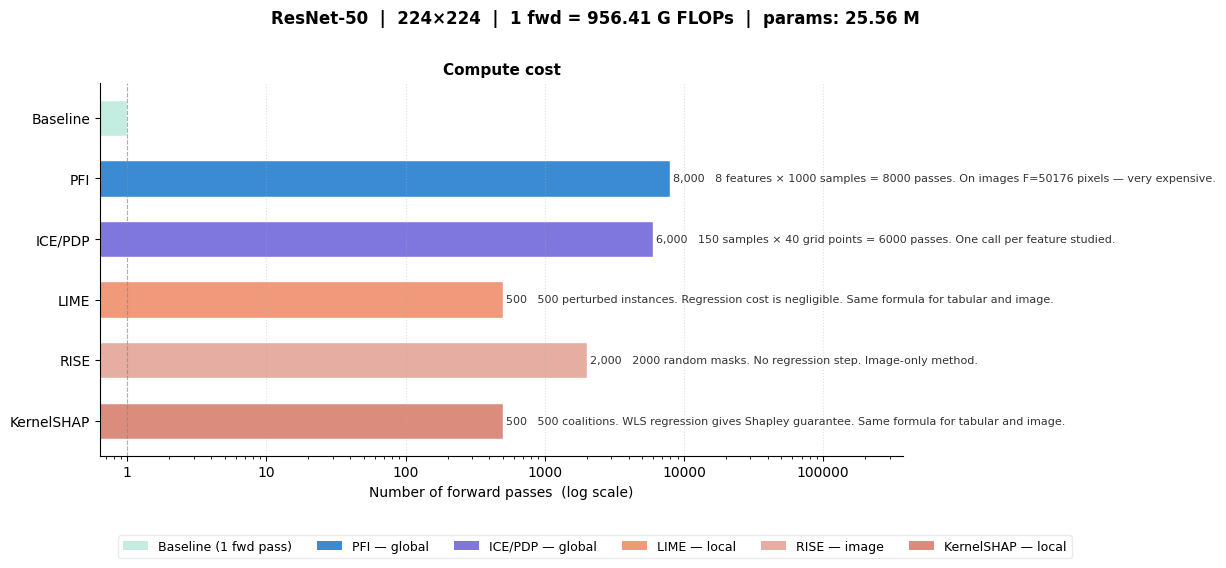
Class 1: 0.020B.4 Complexity estimator of the methods
Perturbation methods scale with the number of forward passes, which depends on the dataset type:
| Method | # Forward passes | Key parameter |
|---|---|---|
| PFI | \(F \times n_{\text{samples}}\) | \(F\) = number of features |
| ICE/PDP | \(N \times G\) | \(G\) = grid resolution |
| LIME (tabular/image) | \(N_{\text{samples}}\) | kernel width controls locality |
| RISE | \(N_{\text{masks}}\) | more masks = smoother saliency |
| KernelSHAP | \(N_{\text{coalitions}}\) | exact Shapley guarantee |
Unlike gradient methods (whose cost scales with model depth), perturbation cost is independent of model architecture.
# !pip install ipywidgets matplotlib thop# ============================================
# Imports
# ============================================
import warnings, math
from dataclasses import dataclass
from typing import Dict, List
import ipywidgets as widgets
import matplotlib.pyplot as plt
import matplotlib.ticker as mticker
import torchvision.models as tvm
from IPython.display import display, clear_output
from matplotlib.patches import Patch
warnings.filterwarnings('ignore')
try:
from thop import profile as thop_profile
HAS_THOP = True
except ImportError:
HAS_THOP = False
# ============================================
# Implementation of DashApp #3
# ============================================
RUN_APP = False # Set to True to run the interactive app
# ── Color scheme ──────────────────────────────
METHOD_COLORS = {
'Baseline': '#C4EDE2',
'PFI': '#3B8BD4',
'ICE/PDP': '#7F77DD',
'LIME': '#F0997B',
'RISE': '#E6ADA2',
'KernelSHAP': '#DC8C7D',
}
LEGEND_ELEMENTS = [
Patch(facecolor='#C4EDE2', label='Baseline (1 fwd pass)'),
Patch(facecolor='#3B8BD4', label='PFI — global'),
Patch(facecolor='#7F77DD', label='ICE/PDP — global'),
Patch(facecolor='#F0997B', label='LIME — local'),
Patch(facecolor='#E6ADA2', label='RISE — image'),
Patch(facecolor='#DC8C7D', label='KernelSHAP — local'),
]
@dataclass
class ModelSpec:
name: str
factory: object
in_ch: int = 3
MODEL_REGISTRY: Dict[str, ModelSpec] = {
'TinyNet (MNIST)': ModelSpec('TinyNet', lambda: TinyNet(), in_ch=1),
'ResNet-18': ModelSpec('ResNet-18', lambda: tvm.resnet18(weights=None)),
'ResNet-50': ModelSpec('ResNet-50', lambda: tvm.resnet50(weights=None)),
'VGG-16': ModelSpec('VGG-16', lambda: tvm.vgg16(weights=None)),
'MobileNetV2': ModelSpec('MobileNetV2',lambda: tvm.mobilenet_v2(weights=None)),
'EfficientNet-B0': ModelSpec('EfficientNet-B0', lambda: tvm.efficientnet_b0(weights=None)),
}
SIZE_OPTIONS = {
'28×28 (MNIST)': 28, '32×32 (CIFAR)': 32,
'64×64': 64, '112×112': 112,
'224×224 (ImageNet)': 224, '384×384': 384, '512×512': 512,
}
def count_params(model):
return sum(p.numel() for p in model.parameters())
def count_flops(model, in_ch, H, W):
dummy = torch.zeros(1, in_ch, H, W)
if HAS_THOP:
try:
macs, _ = thop_profile(model, inputs=(dummy,), verbose=False)
return int(macs)
except Exception:
pass
total = 0
for m in model.modules():
if isinstance(m, nn.Conv2d):
Ho = math.floor((H + 2*m.padding[0] - m.dilation[0]*(m.kernel_size[0]-1) - 1)/m.stride[0] + 1)
Wo = math.floor((W + 2*m.padding[1] - m.dilation[1]*(m.kernel_size[1]-1) - 1)/m.stride[1] + 1)
total += (m.in_channels//m.groups)*m.kernel_size[0]*m.kernel_size[1]*m.out_channels*Ho*Wo
elif isinstance(m, nn.Linear):
total += m.in_features * m.out_features
return total
@dataclass
class MethodComplexity:
name: str
n_forward_passes: float
notes: str
def compute_complexities(spec, H, W,
F_tab=8, N_pfi_samples=1000,
N_ice=150, G=40,
N_lime=500, N_rise=2000,
N_shap=500):
model = spec.factory()
model.eval()
flops = count_flops(model, spec.in_ch, H, W)
n_params = count_params(model)
del model
px = H * W
methods = [
MethodComplexity(
'PFI',
float(F_tab * N_pfi_samples),
f'{F_tab} features × {N_pfi_samples} samples = {F_tab*N_pfi_samples} passes.'
f' On images F={px} pixels — very expensive.',
),
MethodComplexity(
'ICE/PDP',
float(N_ice * G),
f'{N_ice} samples × {G} grid points = {N_ice*G} passes.'
f' One call per feature studied.',
),
MethodComplexity(
'LIME',
float(N_lime),
f'{N_lime} perturbed instances. Regression cost is negligible.'
f' Same formula for tabular and image.',
),
MethodComplexity(
'RISE',
float(N_rise),
f'{N_rise} random masks. No regression step.'
f' Image-only method.',
),
MethodComplexity(
'KernelSHAP',
float(N_shap),
f'{N_shap} coalitions. WLS regression gives Shapley guarantee.'
f' Same formula for tabular and image.',
),
]
return flops, n_params, methods
def human(n):
for u, t in [('G', 1e9), ('M', 1e6), ('K', 1e3)]:
if abs(n) >= t: return f'{n/t:.2f} {u}'
return str(n)
def plot_complexity(flops, n_params, methods, model_name, H, W):
labels = ['Baseline'] + [m.name for m in methods]
vals = [1.0] + [m.n_forward_passes for m in methods]
colors = [METHOD_COLORS.get(l, '#999') for l in labels]
fig, ax = plt.subplots(figsize=(12, 5))
fig.suptitle(
f'{model_name} | {H}×{W} | '
f'1 fwd = {human(flops)} FLOPs | params: {human(n_params)}',
fontsize=12, fontweight='bold', y=1.01,
)
bars = ax.barh(labels, vals, color=colors, edgecolor='white', height=0.6)
ax.set_xscale('log')
ax.set_xlabel('Number of forward passes (log scale)', fontsize=10)
ax.set_title('Compute cost', fontsize=11, fontweight='bold')
ax.xaxis.set_major_formatter(mticker.FuncFormatter(lambda x, _: f'{x:g}'))
ax.axvline(1, color='grey', linestyle='--', linewidth=0.8, alpha=0.6)
for bar, val, m in zip(bars[1:], vals[1:], methods):
ax.text(val*1.05, bar.get_y()+bar.get_height()/2,
f'{val:,.0f} {m.notes}',
va='center', ha='left', fontsize=8, color='#333')
ax.invert_yaxis()
ax.grid(axis='x', linestyle=':', alpha=0.4)
ax.spines[['top', 'right']].set_visible(False)
ax.set_xlim(right=ax.get_xlim()[1] * 30) # room for notes
fig.legend(handles=LEGEND_ELEMENTS, loc='lower center', ncol=6,
bbox_to_anchor=(0.5, -0.10), fontsize=9, framealpha=0.4)
plt.tight_layout()
plt.show()
def show_complexity():
slider_kw = dict(style={'description_width':'120px'},
layout=widgets.Layout(width='360px'),
continuous_update=False)
w_model = widgets.Dropdown(options=list(MODEL_REGISTRY), value='ResNet-50',
description='Model:',
style={'description_width':'80px'},
layout=widgets.Layout(width='280px'))
w_size = widgets.Dropdown(options=list(SIZE_OPTIONS), value='224×224 (ImageNet)',
description='Input size:',
style={'description_width':'80px'},
layout=widgets.Layout(width='280px'))
w_ftab = widgets.IntSlider(value=8, min=1, max=100, step=1,
description='PFI features (tabular):', **slider_kw)
w_npfi = widgets.IntSlider(value=1000, min=100, max=5000, step=100,
description='PFI samples:', **slider_kw)
w_nice = widgets.IntSlider(value=150, min=20, max=500, step=10,
description='ICE samples:', **slider_kw)
w_grid = widgets.IntSlider(value=40, min=5, max=100, step=5,
description='ICE grid points:', **slider_kw)
w_nlime = widgets.IntSlider(value=500, min=50, max=2000, step=50,
description='LIME samples:', **slider_kw)
w_nrise = widgets.IntSlider(value=2000, min=100, max=5000, step=100,
description='RISE masks:', **slider_kw)
w_nshap = widgets.IntSlider(value=500, min=50, max=2000, step=50,
description='SHAP coalitions:', **slider_kw)
w_out = widgets.Output()
def recompute(*_):
spec = MODEL_REGISTRY[w_model.value]
H = W = SIZE_OPTIONS[w_size.value]
with w_out:
clear_output(wait=True)
flops, n_params, methods = compute_complexities(
spec, H, W,
F_tab=w_ftab.value, N_pfi_samples=w_npfi.value,
N_ice=w_nice.value, G=w_grid.value,
N_lime=w_nlime.value, N_rise=w_nrise.value,
N_shap=w_nshap.value,
)
plot_complexity(flops, n_params, methods, spec.name, H, W)
for w in (w_model, w_size, w_ftab, w_npfi, w_nice,
w_grid, w_nlime, w_nrise, w_nshap):
w.observe(recompute, names='value')
ui = widgets.VBox([
widgets.HTML("<h3 style='margin-bottom:4px'>Perturbation Method Complexity Estimator</h3>"),
widgets.HTML("<hr style='margin:4px 0'>"),
widgets.HBox([w_model, w_size]),
widgets.HBox([w_ftab, w_npfi]),
widgets.HBox([w_nice, w_grid]),
widgets.HBox([w_nlime, w_nrise]),
widgets.HBox([w_nshap]),
widgets.HTML("<hr style='margin:4px 0'>"),
w_out,
], layout=widgets.Layout(padding='12px'))
display(ui)
recompute()
if RUN_APP:
show_complexity()# ============================================
# Static Preview: XAI Method Complexity Explorer
# ============================================
# This cell provides a *static snapshot* of the perturbation-based
# explainability complexity analysis framework.
#
import numpy as np
# --- Select a configuration ---
model_name = "ResNet-50"
H = W = 224
spec = MODEL_REGISTRY[model_name]
# --- Compute complexity for default settings ---
flops, n_params, methods = compute_complexities(spec, H, W)
# --- Print summary ---
print("\n=== Static XAI Complexity Snapshot ===\n")
print(f"Model: {model_name}")
print(f"Input resolution: {H}×{W}")
print(f"Parameters: {human(n_params)}")
print(f"Baseline FLOPs (1 forward pass): {human(flops)}\n")
# --- Visualization ---
plot_complexity(flops, n_params, methods, model_name, H, W)
=== Static XAI Complexity Snapshot ===

Model: ResNet-50
Input resolution: 224×224
Parameters: 25.56 M
Baseline FLOPs (1 forward pass): 956.41 G
Additional comment:
- All implementations are intentionally didactic, i.e. optimised for clarity, not speed. Production libraries (
shap,lime,captum) are far more efficient and handle edge cases.