3 Efficient and Reliable LLM Pretraining

3.1 Parallelism Strategies and Scaling Techniques

Modern machine learning models have grown rapidly in both parameter count and computational complexity. Large language models and multimodal architectures usually exceed the memory capacity of a single accelerator and require training times that are impractical without large-scale parallel computation. As a result, parallelization strategies are no longer an optimization detail but a fundamental design choice in large scale training systems.

The objectives of the different approaches of parallelism in modern machine learning are two-fold:

Speed-up the training process by using more resources (GPUs or in general accelerators)
Enable the training of large models that would otherwise be infeasible due to memory constraints (e.g., because of the number of parameters or the context length).

Achieving these goals requires balancing computation, memory, and communication. While adding more GPUs increases available compute and memory capacity, it also introduces non-negligible communication overheads and synchronization costs. The effectiveness of a parallelization strategy therefore depends not only on how work is distributed, but also on how efficiently communication is overlapped with computation and how redundancy in the training state is managed.

Redundancy in the training state takes several distinct forms, and different parallelism strategies target different subsets of it:

Model weights — replicated across devices in plain data parallelism.
Gradients — produced during the backward pass, one value per weight.
Optimizer states — extra per-parameter buffers such as the momentum and variance maintained by Adam.
Activations — the intermediate outputs of each layer that must be retained for backpropagation.

Redundancy in the training state takes several distinct forms, and different parallelism strategies target different subsets of it:

Model weights — replicated across devices in plain data parallelism.
Gradients — produced during the backward pass, one value per weight.
Optimizer states — extra per-parameter buffers such as the momentum and variance maintained by Adam.
Activations — the intermediate outputs of each layer that must be retained for backpropagation.

Three primary axes define the efficiency of large-scale training systems:

Memory usage. Memory is a hard constraint. If a single training step cannot fit within the available device memory, training is impossible. Many scaling techniques exist primarily to reduce peak memory usage or to redistribute memory requirements across devices.
Throughput and utilization. Modern accelerators provide massive computational power, but their effectiveness depends on minimizing idle time. Any time spent waiting—on data transfers, synchronization, or other devices—reduces throughput and wastes electricity. Effective scaling strategies aim to maximize useful computation per unit of time.
Communication. Distributing work across devices means exchanging data between them (gradients, activations, parameters). Communication competes with computation for time and is bounded by interconnect bandwidth and latency; the art of scaling is largely about minimizing it and overlapping what remains with computation.

These axes are deeply intertwined. Improvements along one dimension often come at the expense of another: for example, recomputation trades extra compute for reduced memory usage, while certain forms of parallelism trade memory savings for increased communication. Successful large-scale training is about finding the right balance among memory, computation, and communication for a given hardware setup.

3.2 A High-Level Map of Parallelism

Before diving into the details, it helps to have the whole landscape in view. Every parallelism technique can be understood by asking a single question: what does it shard, and which redundancy does it remove? The table below summarizes the main axes; the rest of the chapter builds them up one at a time, starting from a single GPU.

Parallelism	What it shards / distributes	Redundancy or limit addressed
Data Parallelism (DP)	the batch (a different micro-batch per GPU)	throughput — processes more data in parallel
ZeRO / FSDP	optimizer states, gradients, parameters across DP ranks	memory redundancy of replicated training state
Tensor Parallelism (TP)	weights and the hidden dimension within a layer	per-layer weight and activation memory
Sequence Parallelism (SP)	activations along the sequence dimension in non-TP regions	activation memory of LayerNorm / Dropout
Context Parallelism (CP)	the sequence dimension across the whole model (incl. attention)	activation memory for very long sequences
Pipeline Parallelism (PP)	the model’s layers (depth) across GPUs	parameter memory of very large models
Expert Parallelism (EP)	the experts (feed-forward networks) of an MoE layer	parameter memory / capacity of MoE models

Two of these are sometimes named after the level at which they cut the model: tensor parallelism is intra-layer parallelism (a single layer is split across GPUs), while pipeline parallelism is inter-layer parallelism (different layers live on different GPUs). In practice, state-of-the-art systems combine several of these axes; the closing section discusses how they interact.

3.2.1 First Steps: Training on a Single GPU

Before scaling out to multiple accelerators, it is essential to understand the basic structure and constraints of training on a single GPU. Even the most advanced distributed strategies are built on top of these fundamentals.

At its core, a training step consists of three phases:

Forward pass: inputs are propagated through the model to produce outputs, and the loss is computed at the end from those outputs.
Backward pass: gradients of the loss with respect to model parameters are computed.
Optimization step: parameters are updated using the computed gradients.

These phases are common to virtually all neural network training regimes that involve gradient-based optimization. In practice, these phases may be interleaved, repeated, or partially recomputed, as we will see in the following.

Conceptually, the model can be viewed as a sequence of layers. During the forward pass, intermediate activations are produced at each layer. During the backward pass, gradients corresponding to each layer are computed, often using those stored activations.

Figure 1: Training Step Phases.

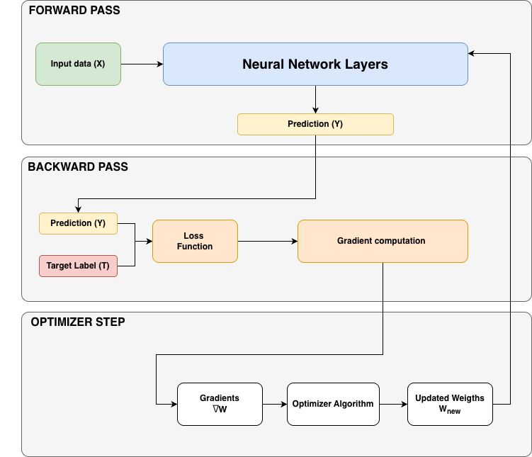
Training step phases: forward pass produces predictions and the loss, backward pass produces gradients, the optimizer updates the weights

During the forward pass, predictions are computed from the inputs and the loss is evaluated at the end. During the backward pass, gradients of the loss with respect to the parameters are computed. During the optimizer step, the weights are updated using those gradients ($W_{new} \leftarrow W_{old} - \eta\,\nabla_W L$).

3.2.2 Batch size

The batch size is one of the most important hyperparameters in model training, and it corresponds to the number of examples in a batch, i.e. the number of samples the model processes at each iteration. It directly affects both optimization dynamics and system-level performance. Ideally batch size should be as large as possible to provide accurate gradient estimates. However, hardware memory constraints often limit the maximum feasible batch size.

Small batch sizes introduce noise into the gradient estimates. Early in training this noise can be advantageous: it helps the optimizer explore the loss landscape and escape sharp or poor local minima. The same high gradient variance, however, slows convergence toward an optimum — small batches may therefore require more optimization steps to converge, and late in training the noise can prevent the model from reaching its best possible performance. (McCandlish et al. 2018)

At the opposite extreme, very large batch sizes produce more accurate gradient estimates but can be inefficient in terms of data usage. Each optimization step consumes many tokens or, in general, samples, thus potentially slowing convergence and wasting compute. Empirically, there is usually a broad “sweet spot” where batch size can vary significantly without materially affecting final model quality.

In large-scale language model training, batch size is commonly expressed in terms of tokens rather than samples. This convention makes training configurations independent of the exact sequence length used.

For single-device training, the relationship is straightforward:

\[\text{batch size (tokens)} = \text{batch size (samples)} \times \text{sequence length}\]

Recent large-scale training runs typically operate with global batch sizes ranging from a few million to several tens of millions of tokens. Over time, both batch sizes and total training corpus sizes have steadily increased, reflecting improvements in hardware and scaling techniques.

E.g. OLMO 3 used a global batch size of ~ 4M tokens for the 7B model and of ~ 8M tokens for the 32B model (Ettinger et al. 2025).

As batch sizes and sequence lengths grow, we quickly encounter a fundamental limitation: GPU memory. Even before introducing multiple devices, memory constraints often prevent us from using the batch sizes we ideally want.

Memory Usage in Transformer Training

In this guide, LLM training is discussed in the context of transformer architectures. While many of the principles discussed here generalize to other architectures, we will focus on transformers for concreteness. During training, several major categories of data must reside in memory. These include, but are not limited to:

Model parameters (mostly weights)
Gradients
Optimizer states
Activations needed for backpropagation

In addition, there is some overhead from CUDA kernels, buffers, and fragmentation. Concretely, this includes the CUDA context and per-kernel workspaces (e.g. scratch space for cuDNN/cuBLAS and reduction kernels), communication buffers reserved by NCCL, and memory fragmentation — free memory split into blocks too small to satisfy a new allocation, which arises when tensors of varying sizes are repeatedly allocated and freed. These contributions are non-negligible in practice (they can account for a few percent to over ten percent of device memory and are a common cause of out-of-memory errors near the limit), but they are hard to model precisely and relatively small compared to the categories above, so we won’t account for them explicitly in this guide.

All of these items are stored as tensors whose sizes depend on model hyperparameters such as hidden dimension, number of layers, sequence length, batch size, and numerical precision (FP32, BF16, FP8, etc.). Precision directly affects memory usage, since it determines how many bytes are required per value.

Memory for Parameters, Gradients, and Optimizer States

For transformer-based language models, the total parameter count is dominated by terms that scale quadratically with the hidden dimension. As models grow, these terms quickly become the main contributors to the total size.

Once the parameter count is known, estimating memory usage for parameters, gradients, and optimizer states is relatively straightforward: multiply parameter count by the number of bytes required per parameter.

In full-precision (FP32) training:

Parameters require 4 bytes each
Gradients require 4 bytes each
Adam optimizer states (momentum and variance) require an additional 8 (4+4) bytes per parameter

Mixed-precision training, which is standard today, shifts this balance. Most computations use BF16, reducing the memory footprint of activations and gradients, while maintaining FP32 “master weights” and optimizer states for numerical stability. Importantly, mixed precision does not reduce the total memory used by parameters and optimizer states—in fact, it often increases it due to the need to maintain multiple copies of the weights. It improves compute efficiency and reduces activation memory.

As a result, even models on the order of a few billion parameters can exceed the memory capacity of a single modern GPU once optimizer states are included. This reality motivates many of the distributed techniques discussed in the rest of this chapter.

Memory for Activations

Activations are the most dynamic and input-dependent part of the memory footprint. Unlike parameters and optimizer states, activation memory scales with both batch size and sequence length.

A key observation is that activation memory grows:

Linearly with batch size
Quadratically with sequence length

The quadratic growth comes specifically from attention: computing $\text{Softmax}(QK^\top/\sqrt{d})$ requires the score matrix $QK^\top$, whose size is $\text{seq\_len} \times \text{seq\_len}$ per head. Doubling the sequence length therefore quadruples this term.

This makes long-context training particularly challenging. For short sequences, activation memory is often negligible compared to parameters. For longer sequences or larger batches, activations quickly dominate the memory budget and become the primary obstacle to scaling.

This “activation explosion” is one of the central problems addressed by modern training techniques. Note that the quadratic term no longer holds with FlashAttention / memory-efficient attention (Dao et al. 2022), where the full $QK^\top$ matrix is never materialized and attention activation memory becomes linear in sequence length.

Gradient Checkpointing (Activation Recomputation)

Gradient Checkpointing (also known as Activation recomputation, or rematerialization) (Korthikanti et al. 2022) is one of the most important tools for controlling memory usage in large-scale training.

The idea is simple: instead of storing all intermediate activations during the forward pass, we selectively discard some of them and recompute them during the backward pass when they are needed. This trades additional computation for a significant reduction in memory usage.

Without recomputation, every intermediate activation between learnable operations must be stored. With recomputation, only a subset of activations—called checkpoints—are retained. During backpropagation, missing activations are reconstructed by rerunning parts of the forward pass.

Two common strategies are used in practice:

Full recomputation: checkpoint only at layer boundaries. This minimizes memory usage but significantly increases compute cost.
Selective recomputation: checkpoint only the most expensive or memory-efficient components. In practice, attention operations are often recomputed (as they grow quadratically with sequence length and are cheap to recompute) while feedforward activations are stored, achieving large memory savings with minimal additional compute.

Modern kernels such as FlashAttention (Dao et al. 2022) integrate selective recomputation by default, so many training setups already benefit from this technique implicitly. FlashAttention is in fact a close analogue of gradient checkpointing applied inside the attention operation: rather than storing the full $\text{seq\_len} \times \text{seq\_len}$ score matrix, it recomputes attention block-by-block during the backward pass, never loading the entire $QK^\top$ matrix into memory.

Overall, recomputation trades additional compute for reduced memory usage. It slightly increases total FLOPs, but the reduced memory pressure and memory bandwidth usage often improve end-to-end training throughput.

Gradient Accumulation

Even with recomputation, activation memory still scales linearly with batch size. Gradient accumulation provides a complementary solution.

Instead of processing the entire batch at once, we split it into micro-batches. Each micro-batch performs its own forward and backward pass, accumulating gradients in buffers that persist across steps. After a fixed number of micro-batches, the optimizer updates the parameters using the averaged gradients.

Let:

mbs be the micro-batch size
grad_acc be the number of accumulation steps

Then the global batch size is:

\[ \text{global batch size} = \text{mbs} \times \text{grad\_acc} \]

Gradient accumulation allows the global batch size to grow arbitrarily large while keeping memory usage roughly constant, since only one micro-batch’s activations are stored at any time.

The trade-off is increased computation per optimizer step, as multiple forward and backward passes are required. Nevertheless, gradient accumulation is widely used because it is simple and effective.

Crucially, gradient checkpointing and gradient accumulation are complementary and can be combined: checkpointing reduces the activation memory of each micro-batch (addressing long sequences), while accumulation reduces the memory tied to the overall batch size (addressing large batches). Together they make it possible to train with both large sequences and large batches on a single device — and both techniques carry over directly to the distributed settings discussed next.

3.3 Data Parallelism (DP)

Data parallelism (DP) scales training by replicating the full model across multiple GPUs—called model replicas—and processing different micro-batches of data in parallel on each GPU. Each replica performs its own forward and backward pass, which increases throughput by exploiting data-level parallelism.

Because each GPU sees different data, it produces different gradients. To keep all replicas synchronized, gradients are averaged across GPUs using a collective communication operation called all-reduce, which is executed during the backward pass, before the optimizer update.

Figure 2: Data Parallelism Workflow.

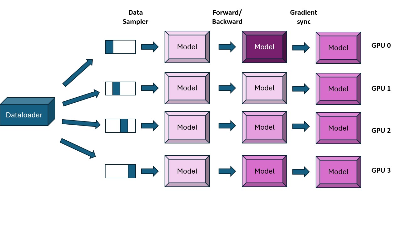
Data parallelism: each GPU holds a full model replica and processes a distinct micro-batch; gradients are synchronized via all-reduce

Each GPU processes a distinct micro-batch with its own full copy of the model. Gradients are synchronized via an all-reduce during the backward pass, so all replicas perform an identical optimizer update.

Worked example (DP, 4 GPUs). With a micro-batch of 4 samples per GPU and dp = 4, GPU 0 processes samples 0–3, GPU 1 samples 4–7, GPU 2 samples 8–11, and GPU 3 samples 12–15. Each GPU holds a full copy of the weights and computes its own gradients; an all-reduce then averages the four gradient sets so that every GPU ends the step with identical, updated weights.

This distributed communication primitive poses a performance challenge as communication can stall computation if handled naively.

Naive Data Parallelism and Its Limitations

A naive DP implementation waits for the full backward pass to finish, then performs a single all-reduce over all gradients. This leads to strictly sequential phases—compute first, then communicate—which leaves GPUs idle during synchronization. This pattern severely limits scalability and must be avoided. (Note that the all-reduce being after the backward pass is precisely the naive behaviour; the optimizations below move it into the backward pass.)

The key optimization principle is therefore:

Overlap communication with computation whenever possible.

Optimization 1: Overlap Gradient Synchronization with Backward Pass

Gradients are produced layer by layer during the backward pass, starting from the last layer and moving backward through the model. Importantly, gradients for later layers become available while earlier layers are still computing.

This allows us to start all-reduce operations as soon as individual gradients are ready, instead of waiting for the entire backward pass to complete. In practice, this is implemented by attaching all-reduce hooks to parameters so that synchronization is triggered immediately when a gradient is computed.

By overlapping gradient communication with ongoing backward computation, most of the synchronization cost is effectively hidden, significantly improving DP efficiency.

Optimization 2: Gradient Bucketing

Communication operations, like GPU kernels, are more efficient when operating on large tensors rather than many small ones. Synchronizing each parameter independently leads to excessive launch overhead and poor bandwidth utilization.

To address this, gradients are grouped into buckets, and a single all-reduce is launched per bucket instead of per parameter. This reduces the number of communication calls and improves bandwidth efficiency—much like packing items into a few large boxes instead of shipping many small ones.

Gradient bucketing is now standard in most distributed training frameworks.

Optimization 3: Interaction with Gradient Accumulation

When gradient accumulation is used, multiple forward/backward passes occur before an optimizer step. A naive DP setup would synchronize gradients after every backward pass, which is unnecessary and wasteful.

Instead, gradient synchronization should only occur after the final accumulation step. In PyTorch, this is typically implemented using model.no_sync(), which temporarily disables all-reduce during intermediate backward passes.

This ensures correctness while minimizing redundant communication.

Note on Communication Buffers

For efficient communication, tensors must be contiguous in memory. Distributed training frameworks therefore often preallocate large contiguous buffers for gradients or parameters. While this improves communication performance, it can slightly increase peak memory usage and must be accounted for in memory planning.

Revisiting Global Batch Size

With both data parallelism and gradient accumulation in play, the global batch size becomes:

\[ \text{global batch size} = \text{mbs} \times \text{grad\_acc} \times \text{dp} \]

where:

mbs is the micro-batch size per GPU
grad_acc is the number of gradient accumulation steps
dp is the number of data-parallel replicas

Given a target global batch size, we can trade off data parallelism against gradient accumulation.

In practice, it is preferable to maximize dp first, since it provides true parallelism. Gradient accumulation is then used only when GPU count is insufficient to reach the desired global batch size.

Data Parallelism as 1D Parallelism:

Data parallelism gives us our first scaling dimension and is therefore referred to as 1D parallelism. It parallelizes over data samples while keeping the model fully replicated.

Practical Recipe for Data-Parallel Training

A typical workflow for setting up data-parallel training, as proposed in (Tazi et al. 2025), is:

Choose a target global batch size (in tokens) based on prior work or convergence experiments.
Select a sequence length, commonly in the 2–8k token range for pretraining.
Determine the largest micro-batch size that fits on a single GPU.
Set the data-parallel size based on available GPUs.
Use gradient accumulation to make up any remaining difference needed to reach the target global batch size.

Example from the LLM Ultrascale Playbook (Tazi et al. 2025):

Target global batch size: 4M tokens
Sequence length: 4k → 1,024 samples
Micro-batch size per GPU: 2
GPUs available: 128

This requires 4 gradient accumulation steps. With 512 GPUs, the same global batch size can be achieved with no accumulation, resulting in faster training.

Scaling Limits of Data Parallelism

At large GPU counts (hundreds to thousands), data parallelism becomes limited by network latency and coordination overhead. All-reduce operations can no longer be fully overlapped with computation, leading to reduced throughput even though per-GPU memory usage remains constant.

Additionally, data parallelism assumes that at least one sample fits on a single GPU (mbs ≥ 1). This breaks down for very large models, which may not fit even with activation recomputation.

Data parallelism is a powerful and simple first step for scaling training, but it does not solve all problems. When models no longer fit on a single GPU—or when communication overhead dominates—we need more advanced strategies.

The next class of techniques involves splitting model states across devices, either through sharding (e.g., ZeRO, FSDP) or model parallelism (tensor, pipeline, context parallelism). These approaches are complementary and can be combined.

3.4 Zero Redundancy Optimizer (ZeRO) and Fully Sharded Data Parallel (FSDP)

ZeRO (Rajbhandari et al. 2020) is a memory-optimization technique introduced in DeepSpeed to eliminate the redundant replication of model states inherent in data parallel training. While data parallelism improves throughput, it naively duplicates optimizer states, gradients, and parameters across all replicas, quickly exhausting GPU memory. ZeRO addresses this by partitioning these states across the data-parallel (DP) dimension, while preserving the abstraction of training a full model.

ZeRO and FSDP are the same algorithm. Fully Sharded Data Parallelism (FSDP) is PyTorch’s native implementation of the sharding scheme that DeepSpeed introduced as ZeRO. FSDP’s FULL_SHARD mode corresponds to ZeRO-3, while SHARD_GRAD_OP corresponds to ZeRO-2. The differences are practical rather than conceptual — the framework and API (FSDP wraps modules in the model; DeepSpeed uses a configuration file and a training engine), the default communication scheduling, and integration with the rest of the stack — but the underlying partitioning of optimizer states, gradients, and parameters across the data-parallel group is identical.

This partitioning reduces memory usage at the cost of additional communication, which can often be overlapped with computation as seen in the DP optimization sections.

There are three main ZeRO stages, each sharding one more component than the last:

Figure 3: ZeRO-1 — optimizer-state partitioning.

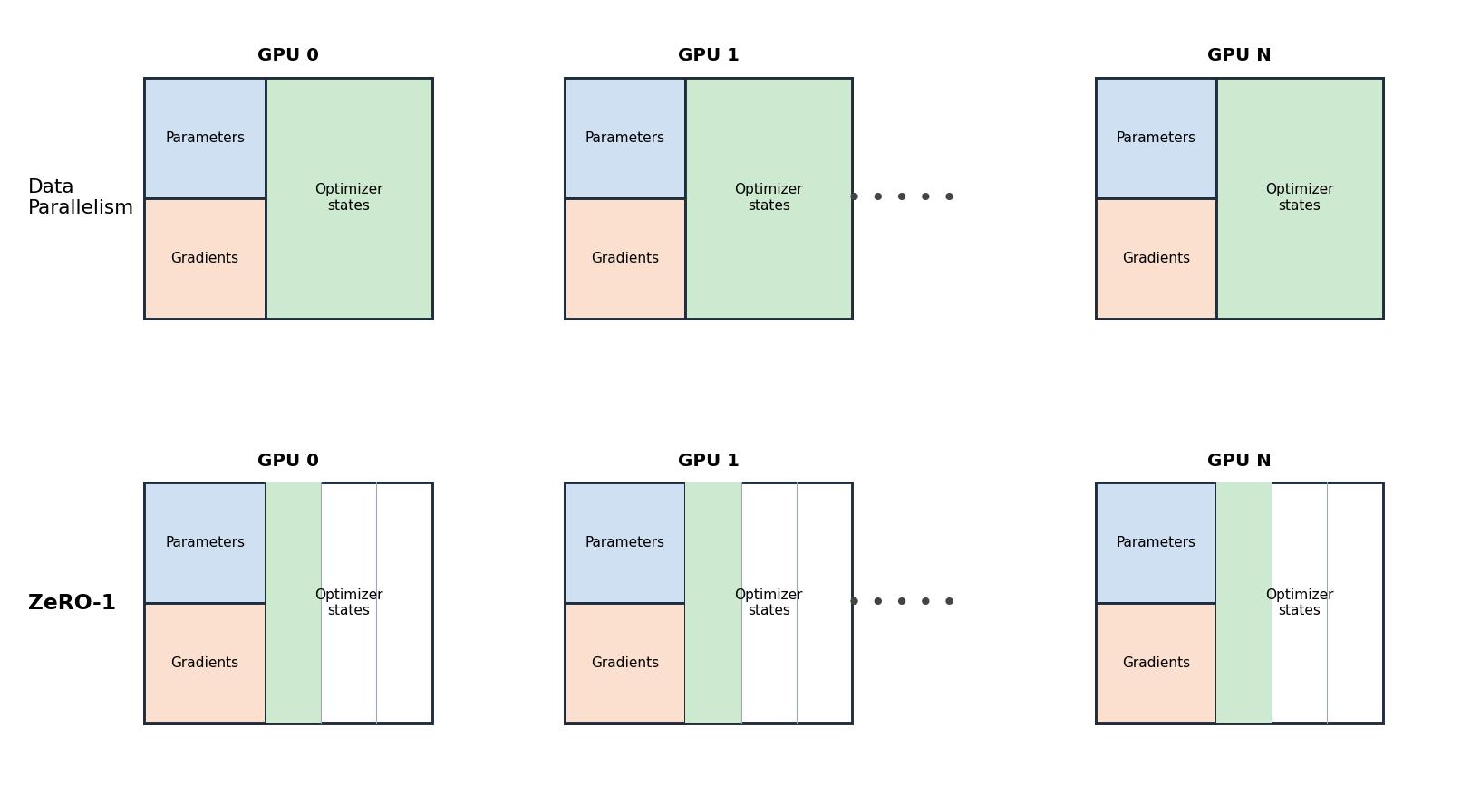
ZeRO-1: optimizer states are sharded across data-parallel GPUs while parameters and gradients stay replicated

ZeRO-1 shards only the optimizer states (Adam momentum and variance) across the data-parallel ranks; parameters and gradients remain fully replicated on every GPU.

Figure 4: ZeRO-2 — optimizer-state + gradient partitioning.

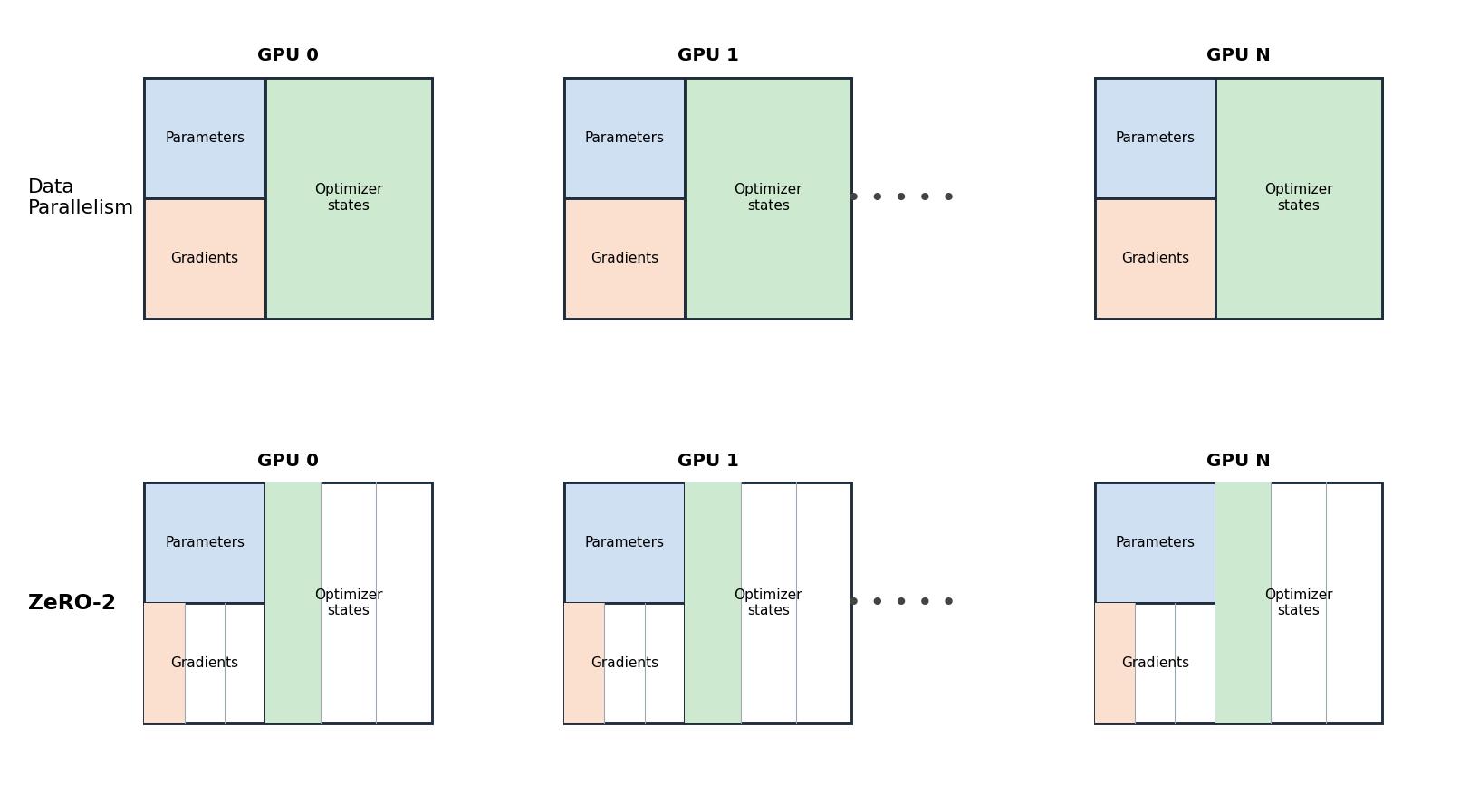
ZeRO-2: optimizer states and gradients are sharded; parameters stay replicated

ZeRO-2 additionally shards the gradients — they are reduce-scattered so each rank keeps only its slice — while parameters remain replicated.

Figure 5: ZeRO-3 — full partitioning.

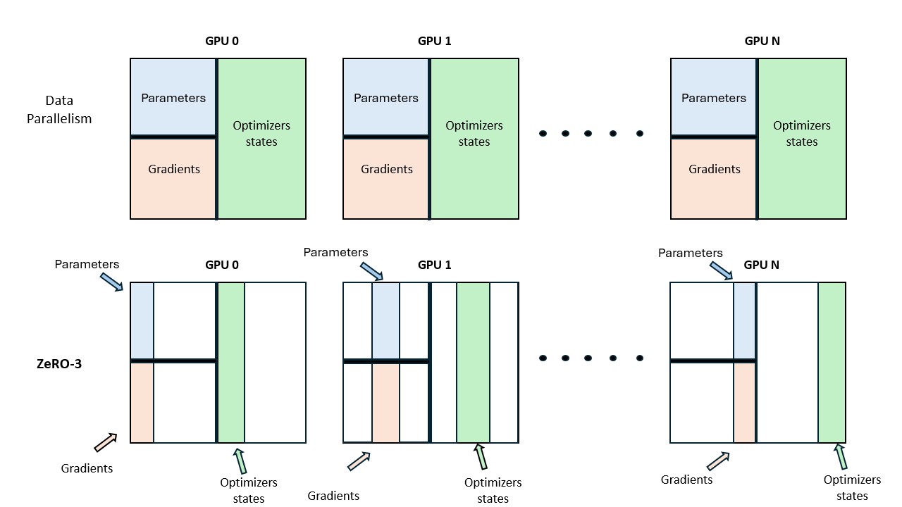
ZeRO-3: optimizer states, gradients, and parameters are all sharded across GPUs

ZeRO-3 shards parameters as well. Full-layer parameters are all-gathered just-in-time for each forward/backward and discarded immediately afterwards. This stage is equivalent to PyTorch FSDP’s FULL_SHARD.

All partitioning is done along the data-parallel axis. Activations are not shardable in ZeRO, since each DP replica processes different inputs and thus already holds unique activations.

The following table summarizes what each stage shards versus replicates, and the communication it adds relative to plain DP:

Stage	Optimizer states	Gradients	Parameters	Communication pattern
Baseline DP	replicated	replicated	replicated	one all-reduce of gradients
ZeRO-1	sharded	replicated	replicated	reduce-scatter gradients + all-gather updated parameters
ZeRO-2	sharded	sharded	replicated	same as ZeRO-1 (gradients reduce-scattered instead of all-reduced)
ZeRO-3	sharded	sharded	sharded	+ all-gather parameters on the fly in both forward and backward

Memory Usage under ZeRO

Let Ψ denote the number of model parameters. In mixed-precision training with Adam (without FP32 gradient accumulation), memory usage is:

Parameters (BF16/FP16): 2Ψ
Gradients (BF16/FP16): 2Ψ
FP32 parameters + optimizer states: 12Ψ

Total (baseline DP): 16Ψ

ZeRO shards these components across N_d data-parallel ranks, reducing memory roughly by a factor of N_d for the sharded components.

We refer the interested reader to the original ZeRO paper (Rajbhandari et al. 2020) for a detailed derivation of memory usage at each stage and to the documentation of DeepSpeed and PyTorch FSDP for additional details on the three stages and their implementation.

Summary: DP + ZeRO

Data parallelism increases throughput by parallelizing over data.
ZeRO eliminates memory redundancy by sharding model states across DP ranks.
ZeRO enables training models that do not fit on a single GPU.
Communication overhead increases from ZeRO-1 → ZeRO-3, but is largely hidden via overlap.

Limitations

Activations are not sharded and still scale with batch size and sequence length.
DP requires each layer to fit on a single GPU.
At large DP scales, communication latency limits efficiency.

3.5 Tensor Parallelism (TP)

Figure 6: Tensor Parallelism.

Tensor parallelism: a weight matrix is split across GPUs and each GPU computes a shard of the matrix multiplication

A linear layer’s weight matrix is split across GPUs; each GPU computes a partial matrix multiplication, and the partial results are combined by a collective operation (all-gather or all-reduce, depending on the split).

Tensor parallelism leverages the mathematical properties of matrix multiplication:

\[A \times B\]

To understand how it works, consider two fundamental ways to decompose this product:

Column-wise decomposition (split $B$ by columns) \[A \cdot B = A \cdot [B_1 \; B_2 \; \cdots] = [AB_1 \; AB_2 \; \cdots]\]
Inner-dimension decomposition (split $A$ by columns and $B$ by rows)

\[A \cdot B = \begin{bmatrix} A_1 & A_2 & \cdots \end{bmatrix} \begin{bmatrix} B_1 \\ B_2 \\ \vdots \end{bmatrix} = \sum_{i=1}^{n} A_i B_i \]

This means we can compute a matrix product either by:

multiplying each column of $B$ independently and concatenating the results, or
splitting along the inner dimension and summing the partial products $A_i B_i$.

In neural-network layers this product is written $X \times W$, where $X$ is the input/activations and $W$ the layer weights; tensor parallelism shards $W$ (and, where appropriate, the corresponding activations) across GPUs according to one of the two decompositions above.

Sharding Strategies in Tensor Parallelism

In TP, tensors are split into $N$ shards along a chosen dimension and distributed across $N$ GPUs.

Column-wise (Column-Linear) Sharding

Inputs are broadcast to all GPUs
Weight matrix is split by columns
Each GPU computes a partial output
Outputs are combined using all-gather

Row-wise (Row-Linear) Sharding

Weight matrix is split by rows
Inputs are scattered: each GPU receives the shard of $X$ that matches its rows of $W$ (i.e. $X$ is split along the inner dimension so that GPU $i$ holds $X_i$ and $W_i$)
Each GPU computes a partial product $X_i W_i$, which is already correctly shaped
The final output is obtained by summing the partial products with an all-reduce

These two sharding methods require different collective communication primitives.

Worked example (TP, 4 GPUs). Consider the MLP $Y = (X W_1)\,W_2$. Split $W_1$ column-wise: GPU $g$ holds the column block $[g\cdot d/4 : (g{+}1)\cdot d/4]$ and, given the broadcast input $X$, computes one quarter of the hidden activations. Then split $W_2$ row-wise to match, so each GPU multiplies its hidden shard by its rows of $W_2$ to produce a partial output; a single all-reduce sums the four partials into $Y$. For multi-head attention with 8 heads, GPU 0 computes heads 0–1, GPU 1 heads 2–3, GPU 2 heads 4–5, and GPU 3 heads 6–7.

3.5.1 Tensor Parallelism in Transformer Blocks

A Transformer layer consists mainly of:

a Multi-Layer Perceptron (MLP) block
a Multi-Head Attention (MHA) block

Feedforward (MLP) Block

An efficient setup is:

Column-linear layer
Row-linear layer

This results in:

broadcast (often implicit during training)
all-reduce at the end

This ordering avoids unnecessary intermediate synchronization (the column-linear output feeds the row-linear layer directly, with no collective in between).

Multi-Head Attention (MHA)

Query (Q), Key (K), and Value (V) projections are column-parallel
Output projection is row-parallel
Each GPU computes attention for a subset of heads

This extends naturally to:

Multi-Query Attention (MQA)
Grouped Query Attention (GQA)

Constraint on TP Degree

The TP degree should not exceed the number of attention heads.

For GQA:

$ $
The number of K/V heads must be divisible by the TP degree

Performance Trade-offs of Tensor Parallelism

Tensor parallelism introduces communication directly into the computation path, making it harder to overlap with compute compared to ZeRO.

Key observations:

Synchronization points (e.g., all-reduce) lie on the critical path
Communication overhead grows rapidly beyond TP > 8
Inter-node communication (e.g., TP=16 or 32) causes steep throughput drops

Despite this, TP provides substantial memory savings by sharding:

parameters
gradients
optimizer states
activations (partially)

3.5.2 Sequence Parallelism (SP)

Sequence parallelism complements TP by sharding activations along the sequence dimension for operations not handled by TP, such as LayerNorm or Dropout.

For a single token, let $x \in \mathbb{R}^{h}$ be its hidden vector, where $h$ is the hidden dimension. LayerNorm normalizes each token over its own features:

\[\text{LayerNorm}(x) = \gamma \cdot \frac{x - \mu}{\sqrt{\sigma^2 + \epsilon}} + \beta, \qquad \mu = \frac{1}{h}\sum_{i=1}^{h} x_i, \quad \sigma^2 = \frac{1}{h}\sum_{i=1}^{h}(x_i - \mu)^2\]

The mean $\mu$ and variance $\sigma^2$ are computed across the hidden dimension of one token — not across the batch, which is what distinguishes LayerNorm from BatchNorm. Consequently, a GPU can normalize a token only if it holds all $h$ features of that token. This is exactly why SP shards along the sequence dimension rather than the hidden dimension: each GPU keeps a subset of tokens (e.g. tokens 0–1023) but the full feature vector for each of them, so LayerNorm and Dropout require no cross-GPU communication. These operations also have no inter-token dependencies — unlike attention, there is no $QK^\top$ term coupling different tokens — so splitting tokens across GPUs is safe. Even though they are cheap compute-wise, they consume significant activation memory, which is what SP reduces.

3.5.3 TP + SP Transitions

Different collective operations are used when moving between TP and SP regions. The operators $f/f^*$ and $g/g^*$ form conjugate pairs: the operator used in the forward pass has a corresponding adjoint in the backward pass.

Forward Pass

$f$: identity operator
$f^*$: all-reduce
$g$: all-gather
$g^*$: reduce-scatter

Backward Pass

$f$: all-reduce
$f^*$: identity operator
$g$: reduce-scatter
$g^*$: all-gather

These conjugate pairs ensure correctness with minimal memory overhead.

Example Flow (TP + SP)

Figure 7: TP + SP Forward Flow.

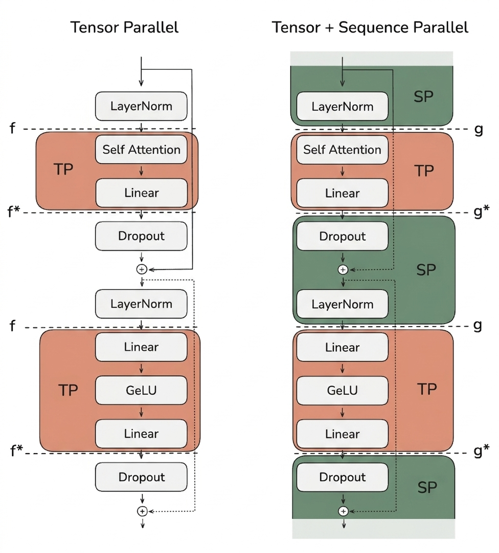
TP + SP flow: activations alternate between sequence-sharded (SP) regions and hidden-sharded (TP) regions, with all-gather and reduce-scatter at the transitions

Activations alternate between SP regions (sharded along the sequence) and TP regions (sharded along the hidden dimension). An all-gather restores the full sequence entering a TP region; a reduce-scatter restores the sequence sharding when leaving it.

SP region (LayerNorm) — Activations split along the sequence dimension
SP → TP transition — All-gather restores the full sequence
TP region (MLP / Attention) — Sharding along the hidden dimension
TP → SP transition — Reduce-scatter restores sequence sharding

This ensures the maximum activation size is reduced to:

\[\frac{b \cdot s \cdot h}{\text{TP}}\]

instead of $b\cdot s \cdot h$, where $b$ is the batch size, $s$ the sequence length, $h$ the hidden dimension, and $\text{TP}$ the tensor-parallel degree.

Worked example (SP, 4 GPUs, 4096 tokens). In the LayerNorm/Dropout regions each GPU owns a slice of the sequence — GPU 0 holds tokens 0–1023, GPU 1 tokens 1024–2047, GPU 2 tokens 2048–3071, GPU 3 tokens 3072–4095 — together with the full hidden vector for each of its tokens, so it computes each token’s mean and variance locally. Entering the TP region, an all-gather reconstructs the full 4096-token sequence on every GPU; leaving it, a reduce-scatter hands each GPU back its 1024-token slice.

Communication Cost Analysis

TP: 2 all-reduces per layer
TP + SP: 2 all-gathers + 2 reduce-scatters per layer

Since:

all-reduce ≈ all-gather + reduce-scatter

→ Total communication cost is equivalent.

However:

Communication cannot be fully overlapped with compute
Performance heavily depends on interconnect bandwidth

Practical Observations

Biggest performance drop: TP=8 to TP=16 (intra-node to inter-node), assuming 8 GPUs per node. On Leonardo we have 4 A100 per node, so TP=4 is intra-node.
TP + SP enables much larger batch sizes and sequence lengths
Typically used within a node (TP ≤ GPUs per node)

Summary

Tensor Parallelism (TP) shards computation along the hidden dimension
Sequence Parallelism (SP) shards the remaining ops along sequence length
TP + SP significantly reduces activation memory
Communication overhead limits scalability
LayerNorm gradients in SP require an all-reduce (minor overhead)

Remaining challenges:

Long sequences → activation blow-up in TP regions
Very large models → inter-node TP slowdown

3.5.4 Context Parallelism (CP)

With tensor parallelism (TP) and sequence parallelism (SP), we can significantly reduce per-GPU memory requirements by distributing both model weights and activations across GPUs. However, when training on very long sequences (e.g., 128k tokens or more), we may still exceed the memory available on a single node. This happens because, inside TP regions, we still need to process the full sequence length.

Even with full activation recomputation (which already incurs a heavy compute overhead of ~30%), we must still keep some boundary activations in memory, and these scale linearly with sequence length.

Core Idea of Context Parallelism

Context parallelism is conceptually similar to sequence parallelism — both split the input along the sequence dimension. The difference is where and how far the split reaches:

Sequence Parallelism (SP): shards the sequence only in the regions not covered by tensor parallelism (e.g. LayerNorm, Dropout); inside TP regions the full sequence is reconstructed via all-gather.
Context Parallelism (CP): shards the sequence across the entire model, including the modules where TP is already applied, and adds the communication needed so that attention still works correctly on the split sequence.

When CP is combined with TP, activations are therefore split along two dimensions at once:

the hidden dimension (by TP)
the sequence dimension (by CP)

This significantly reduces the impact of long sequence lengths on memory usage.

Splitting the sequence dimension:

Does not affect modules like MLPs and LayerNorm, where tokens are processed independently.
Does not require expensive communication for weights, since weights are not split — only the inputs (tokens) are.

Like data parallelism, CP synchronizes gradients using an all-reduce after the backward pass. The reason is that CP replicates the model weights but shards the sequence: every CP rank computes gradients for the same weights, but from different tokens. To obtain a correct update, these per-rank gradients must be averaged across all CP ranks with an all-reduce — exactly as in DP.

Context Parallelism with Attention

In attention layers, each token needs access to key/value (K/V) pairs from all other tokens (or all previous tokens in causal attention). Since CP splits the sequence across GPUs, no single GPU initially has access to all required K/V pairs.

A naive implementation would require massive communication. Fortunately, there is an efficient solution: Ring Attention (Liu et al. 2023).

Ring Attention

Ring Attention (Liu et al. 2023) arranges the CP GPUs in a logical ring. Each GPU holds the queries for its own slice of tokens and, initially, only its own key/value (K/V) block. The GPUs then pass K/V blocks around the ring step by step: at each step a GPU computes the partial attention between its local queries and the K/V block it currently holds, then forwards that block to the next GPU and receives a new one from the previous GPU. Because attention’s softmax can be computed incrementally — using the running-maximum and running-denominator trick of the “online softmax” employed by FlashAttention — these partial results are accumulated into the correct output without ever materializing the full $QK^\top$ matrix. Since each send/receive overlaps with the local attention computation, communication is largely hidden behind compute.

Concretely, assume:

4 GPUs (GPU 0–3) and 4 token blocks (Token 0–3)
GPU $i$ starts with Token $i$ and its $(Q_i, K_i, V_i)$

At each time step, every GPU performs:

Send its current $(K, V)$ block to the next GPU in the ring (non-blocking).
Compute partial attention between its local $Q$ and the $(K, V)$ block it currently holds: \[\text{Softmax}\!\left(\frac{Q K^\top}{\sqrt{d}}\right) \cdot V\]
Receive the next $(K, V)$ block from the previous GPU.
Accumulate the partial result and repeat.

After 4 steps, GPU $i$ has attended to $(K_0,V_0), (K_1,V_1), (K_2,V_2), (K_3,V_3)$ and attention is complete. This pipeline-style exchange forms a ring, hence the name Ring Attention.

Load Imbalance in Naive Ring Attention

In causal attention, the softmax is computed row-wise. This leads to severe load imbalance:

Early GPUs can compute immediately.
Later GPUs must wait for more K/V data.
Some GPUs do significantly less work than others.

This imbalance reduces overall efficiency. To fix it, we can reorder tokens across GPUs so that each GPU receives a mix of early and late tokens. This approach is known as Zig-Zag Attention.

Key properties:

Balanced compute across GPUs
Each GPU eventually needs data from all others
Produces a more uniform effective attention mask

Zig-Zag Attention is closely related to Striped Attention (Brandon et al. 2023). Both rebalance the causal workload that naive Ring Attention leaves uneven, but they differ in the token-permutation pattern: Striped Attention assigns each GPU a strided set of tokens (e.g. GPU $i$ gets tokens $i, i{+}P, i{+}2P, \dots$ for $P$ GPUs), whereas Zig-Zag pairs an early and a late contiguous block on each GPU. Both build directly on Ring Attention and recover near-uniform per-GPU work under a causal mask.

Communication Strategies for Ring Attention

There are two main ways to exchange key/value pairs:

All-Gather Approach
- All GPUs gather all K/V pairs at once.
- Simple to implement.
- Requires large temporary memory.
- Similar to ZeRO-3-style parameter gathering.
All-to-All (Ring) Approach
- GPUs exchange K/V chunks incrementally.
- Much more memory efficient.
- Communication is overlapped with computation.
- Slightly higher base latency due to multiple steps.

Approach	Memory Usage	Complexity	Overlap
All-gather	High	Low	Limited
Ring (A2A)	Low	Higher	Good

In practice, the ring-based all-to-all approach is preferred for long sequences due to its superior memory efficiency.

Summary of Context Parallelism

CP splits activations along the sequence dimension across the entire model.
Most layers work without additional communication.
Attention requires specialized handling via Ring Attention.
Zig-Zag (or Striped) ordering balances computation across GPUs.
Ring-based communication trades complexity for lower memory usage.

Since TP does not scale well across nodes (due to communication latency), if model weights or activations no longer fit on a single node we need pipeline parallelism (PP) as an additional axis of parallelism.

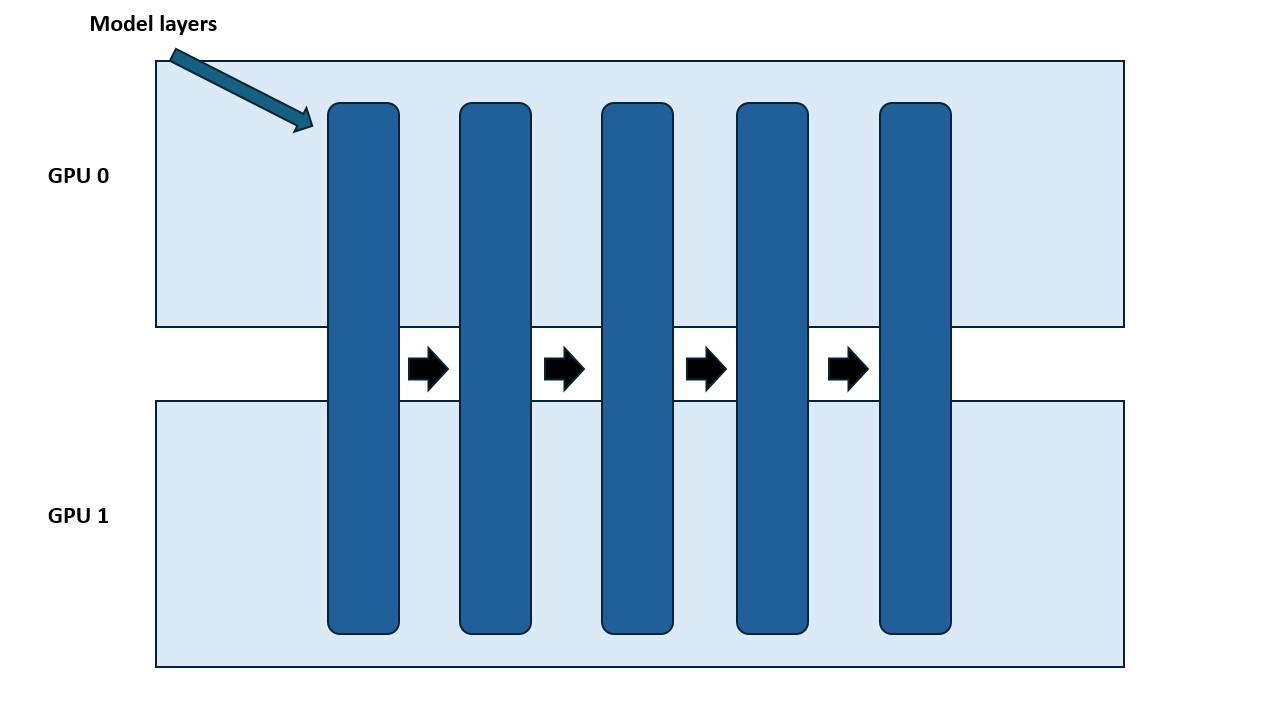
3.5.5 Pipeline Parallelism (PP)

Figure 8: Pipeline Parallelism.

Pipeline parallelism: consecutive layers of the model are assigned to different GPUs, and micro-batches flow through the stages

Consecutive layers of the model are assigned to different GPUs (stages). Micro-batches flow through the stages in sequence on the forward pass and in reverse on the backward pass.

Sequence parallelism and context parallelism help with long sequences, but they don’t address scenarios where the model size itself is the bottleneck. For very large models (70B+ parameters), the weights alone can exceed the memory capacity of a single node. To address this, we introduce another parallelism dimension.

It helps to see how PP fits with the other axes: DP shards the batch; TP shards the weights and the hidden dimension within a layer; SP/CP shard activations along the sequence dimension (and CP also distributes the attention computation); while PP shards the model’s layers (its depth).

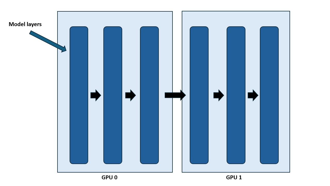
Pipeline parallelism splits the model along its depth, distributing layers across multiple GPUs. For example, with 8 GPUs:

GPU 1 holds layers 1–4
GPU 2 holds layers 5–8

Each GPU only stores and computes a fraction of the model, significantly reducing per-GPU parameter memory.

Worked example (PP, 4 GPUs). Split a 32-layer model into 4 stages: GPU 0 holds layers 1–8, GPU 1 layers 9–16, GPU 2 layers 17–24, and GPU 3 layers 25–32. Micro-batch 0 flows GPU 0 → 1 → 2 → 3 on the forward pass and 3 → 2 → 1 → 0 on the backward pass. While micro-batch 0 is being processed on GPU 1, GPU 0 already begins micro-batch 1, so the stages stay busy.

This approach may remind you of ZeRO-3, which also shards parameters across GPUs. Interestingly, while parameter memory is reduced, activation memory remains roughly unchanged on each GPU. The reason lies in the pipeline schedule, not the layer assignment. Each GPU executes only its own layers; the micro-batches that traverse all stages sequentially. To keep the pipeline full and avoid idling, each stage must hold several micro-batches “in flight” — on the order of $PP$ of them — before the first backward reaches it. Every in-flight micro-batch must retain its activations, so although a GPU owns only $1/PP$ of the layers, it stores activations for $\approx PP$ micro-batches:

\[PP \times (\text{activations per micro-batch} / PP) \approx \text{activations for the full model}\]

As a result, activation memory remains roughly the same as without pipeline parallelism.

Sequential Execution and the Pipeline Bubble

In its simplest form, PP executes layers sequentially across devices, passing activation tensors from one GPU to the next.

Advantages

Low interconnect bandwidth requirements
Communication only happens at layer boundaries
Much cheaper than TP-style intra-layer communication

Disadvantage

Strong sequential dependency between GPUs

This leads to idle GPU time, known as the pipeline bubble, a common pattern in parallel computing.

How much time is spent idle waiting for data from other GPUs?

Let:

$t_f$ = forward time per micro-batch per stage
$t_b$ = backward time per micro-batch per stage (often $t_b \approx 2t_f$)
$p$ = pipeline degree (number of GPUs)

Ideal time: \[t_{id} = t_f + t_b\]

Bubble time: \[t_{pb} = (p - 1)(t_f + t_b)\]

Bubble ratio: \[r_{\text{bubble}} = \frac{t_{pb}}{t_{id}} = p - 1\]

Here the ideal time $t_{id}$ is the useful work time — what processing a micro-batch would take if the pipeline were perfectly full — and is independent of the number of GPUs $p$. The bubble time $t_{pb}$ is the idle GPU-time spent filling and draining the pipeline (measured in GPU-time, e.g. GPU-hours, summed across the idle devices). The bubble ratio expresses how much idle time we pay per unit of useful work; as the pipeline depth $p$ increases, utilization drops sharply.

All Forward, All Backward (AFAB)

We can reduce idle time by splitting batches into micro-batches. While GPU 2 processes micro-batch 1, GPU 1 can already process micro-batch 2. This is known as the All Forward, All Backward (AFAB) schedule: all forward passes for the micro-batches are run first, then all backward passes.

Ideal time for $m$ micro-batches: \[t_{id} = m(t_f + t_b)\]

Bubble ratio: \[r_{\text{bubble}} = \frac{p - 1}{m}\]

Increasing the number of micro-batches reduces the bubble—but introduces a new problem: AFAB requires storing all activations until the backward phase starts, leading to excessive memory usage.

To fix this, we begin backward computation as early as possible.

One Forward, One Backward (1F1B)

The 1F1B schedule alternates forward and backward passes once the pipeline is filled.

Benefits:

Activation memory reduced from $m$ to $p$ micro-batches
Allows more micro-batches → smaller bubble

Drawbacks:

Bubble size unchanged
Complex scheduling
Forward/backward passes are no longer globally synchronized

Interleaved Pipeline Parallelism

To further reduce the bubble, we can interleave stages.

Instead of assigning contiguous layers to each GPU:

GPU 1: layers 1, 3, 5, 7
GPU 2: layers 2, 4, 6, 8

This creates a looping pipeline where micro-batches circulate across GPUs.

Let $v$ be the number of model chunks per GPU.

Bubble time: \[t_{pb} = \frac{(p - 1)(t_f + t_b)}{v}\]

Bubble ratio: \[r_{\text{bubble}} = \frac{p - 1}{v \cdot m}\]

Trade-off:

Smaller bubble
Increased communication (×$v$)
More complex scheduling

Scheduling policies include:

Depth-first — push a micro-batch through all of a GPU’s chunks before starting the next micro-batch, freeing its activation memory as early as possible (lower latency, lower activation memory).
Breadth-first — advance all micro-batches one chunk at a time, keeping the pipeline maximally filled to minimize the bubble (higher throughput, more activation memory).

See Breadth-First Pipeline Parallelism (Lamy-Poirier 2023) for details.

Llama 3.1 Pipeline Schedule

Llama 3.1 uses:

1F1B
Interleaved stages
Tunable depth-first vs breadth-first priority

Figure 9: Llama 3.1 Pipeline Schedule.

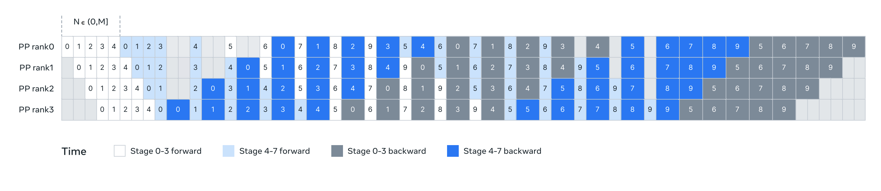
Llama 3.1 interleaved 1F1B pipeline schedule across four pipeline ranks

Illustration of pipeline parallelism in Llama 3. Pipeline parallelism partitions eight pipeline stages (0 to 7) across four pipeline ranks (PP ranks 0 to 3): the GPUs with PP rank 0 run stages 0 and 4, the GPUs with PP rank 1 run stages 1 and 5, and so on. The colored blocks (0 to 9) represent a sequence of micro-batches, where M is the total number of micro-batches and N is the number of continuous micro-batches for the same stage’s forward or backward. The key insight is to make N tunable. (Image source: Llama 3.1 technical report (Grattafiori et al. 2024).)

3.5.6 Zero Bubble and DualPipe

Recent work has pushed pipeline efficiency close to zero bubble, notably in DeepSeek-V3/R1 (DeepSeek-AI 2024).

These methods rely on fine-grained decomposition of the backward pass:

$B$: backward for inputs
$W$: backward for weights

Only $B$ is required to continue backward propagation. $W$ can be scheduled later to fill bubbles.

This idea was formalized in Sea AI Lab’s Zero Bubble work (Qi et al. 2023).

DualPipe (DeepSeek-V3/R1)

DualPipe extends zero-bubble scheduling by:

Running two streams from both ends of the pipeline
Interleaving them to further reduce idle time

Figure 10: DualPipe Scheduling.

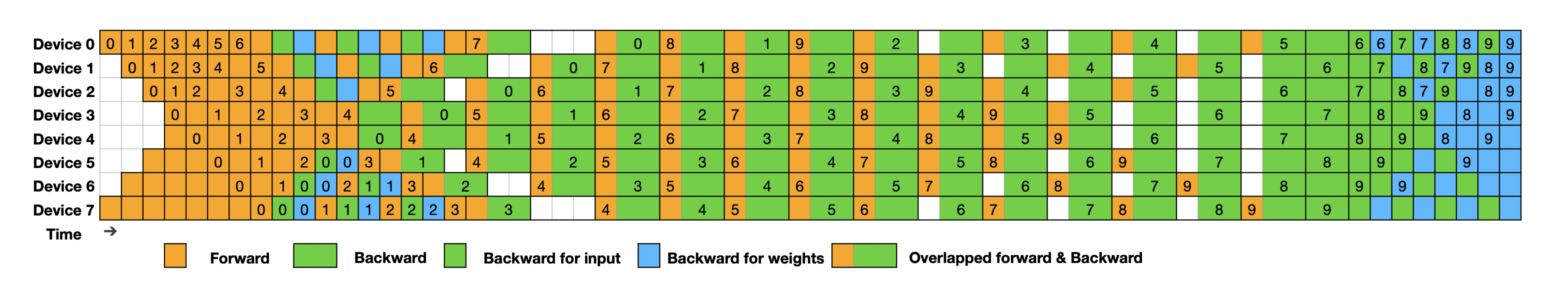
DualPipe scheduling for 8 pipeline ranks and 20 micro-batches running in two directions

Example DualPipe scheduling for 8 PP ranks and 20 micro-batches in two directions. The micro-batches in the reverse direction are symmetric to those in the forward direction, so their batch IDs are omitted for simplicity. Two cells enclosed by a shared black border have mutually overlapped computation and communication. (Image source: DeepSeek-V3 technical report (DeepSeek-AI 2024).)

Optimizing these schedules typically involves:

Measuring fine-grained op durations
Solving an Integer Linear Programming (ILP) problem

Due to their complexity, we won’t provide code examples, but the core ideas should now be clear.

Pipeline Parallelism Summary

Pipeline parallelism shards models by depth
Micro-batching reduces bubbles
1F1B reduces activation memory
Interleaving reduces bubbles further
Zero-bubble and DualPipe push utilization close to optimal

3.5.7 Expert Parallelism (EP)

This is the last parallelism method we’re going to discuss and it is tied to specific LLM architectural choices, as it is used in Mixture of Experts (MoE) models.

The Mixture of Experts paradigm gained significant traction with models such as GPT-4, Mixtral (Jiang et al. 2024), and DeepSeek-V3/R1 (DeepSeek-AI 2024). The core idea is simple: instead of a single feedforward (MLP) module per transformer layer, we introduce multiple experts and dynamically route tokens to a subset of them for processing.

Figure 11: Mixture-of-Experts Layer.

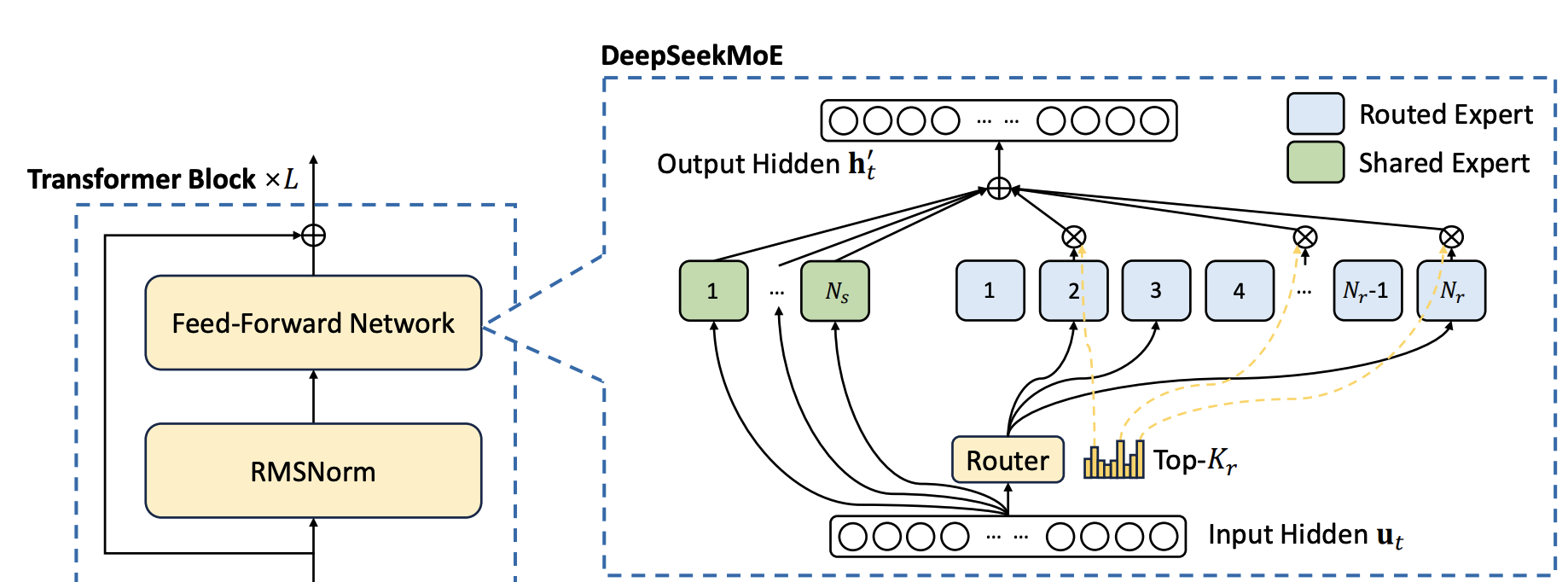
Mixture-of-Experts layer: a router sends each token to a subset of expert feed-forward networks

Scheme of an MoE layer. A router assigns each token to a subset of expert feed-forward networks. (Image source: DeepSeek-V3 technical report (DeepSeek-AI 2024).)

3.5.8 What Is Expert Parallelism?

The structure of MoE layers makes them naturally amenable to expert parallelism (EP). Since each expert’s feedforward network is independent, we can place different experts on different GPUs or workers.

Compared to tensor parallelism:

There is no need to split matrix multiplications
We simply route token hidden states to the appropriate expert

This makes EP significantly more lightweight than TP in terms of implementation and communication complexity.

In practice, EP is almost always combined with data parallelism (DP). The reason is that EP only applies to MoE layers and does not shard input tokens. Without DP, all GPUs would redundantly compute the non-MoE parts of the model.

By combining EP and DP:

DP shards input batches
EP shards experts

This allows efficient utilization of GPUs across both dimensions.

Worked example (EP, 4 GPUs, 8 experts). Place two experts per GPU: GPU 0 holds experts E0–E1, GPU 1 holds E2–E3, GPU 2 holds E4–E5, GPU 3 holds E6–E7. For each token, the router selects its top-$k$ experts and an all-to-all sends the token’s hidden state to the GPUs that own them; e.g. token 0 routed to E3 and E5 is sent to GPU 1 and GPU 2, processed there, and returned by a second all-to-all that restores the original token order.

Figure 12: Expert Parallelism combined with Data Parallelism.

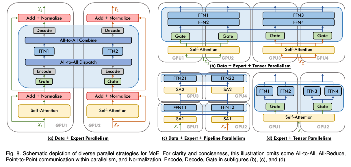
Expert parallelism combined with data parallelism: experts are sharded across GPUs while batches are sharded by DP

Scheme of EP + DP: experts are distributed across GPUs (EP) while input batches are distributed by data parallelism (DP). (Image source: “A Survey on Mixture of Experts” (Cai et al. 2025).)

3.5.9 Practical Design Considerations

Efficient EP is closely tied to model and router design. For example, DeepSeek-V3 enforces a routing constraint that limits each token to at most $M$ nodes (with $M=4$ in their case). This keeps token routing largely within a single node and significantly reduces communication overhead.

While expert parallelism has existed for quite some time, the recent popularity of MoE models has made it a central technique for scaling model capacity.

3.5.10 5D Parallelism Summary and Interactions

This summary concludes the discussion on all five major parallelism strategies used in large-scale model training. Each one removes a specific redundancy or lifts a specific limit — the batch, the weights, the activations (tokens/attention), the model’s layers (feed-forward or expert networks), and the optimizer state (gradients and intermediate states):

Data Parallelism (DP) — batch dimension
Tensor Parallelism (TP) — hidden dimension within a layer
Sequence & Context Parallelism (SP / CP) — sequence length
Pipeline Parallelism (PP) — model layers
Expert Parallelism (EP) — expert dimension

Along with the three ZeRO strategies for memory reduction:

ZeRO-1 — optimizer states
ZeRO-2 — optimizer states + gradients
ZeRO-3 — optimizer states + gradients + parameters

A natural question now arises: how do these methods interact, and which ones combine well together? The tables and diagrams below (source: (Tazi et al. 2025)) summarize these interactions.

Pipeline Parallelism vs ZeRO-3

Both pipeline parallelism and ZeRO-3 partition model weights across GPUs and operate along the model-depth axis, but they do so differently. ZeRO-3 additionally partitions the optimizer states and gradients; pipeline parallelism partitions only whole layers (optimizer states and gradients follow the layers a GPU owns). The crucial difference is what each GPU stores and computes: under ZeRO-3 each GPU stores only a shard of every layer’s parameters and all-gathers them just-in-time to run the full layer, whereas under PP each GPU stores whole layers and runs only those.

Aspect	ZeRO-3	Pipeline Parallelism
Each GPU stores	Shard of every layer	Whole layers (a subset)
Communication	Parameters (all-gather) + gradients (reduce-scatter)	Activations + activation gradients (at stage boundaries)
Orchestration	Model-agnostic	Model-agnostic
Main challenge	Parameter gathering & comms	Efficient scheduling (the bubble)
Scaling preference	Large micro-batch & seq length	Large gradient accumulation

Note that ZeRO-3’s communication involves parameters (all-gathered for each forward/backward) and gradients (reduce-scattered); the optimizer states stay sharded and are not communicated. Pipeline parallelism communicates the activations between stages on the forward pass and their gradients on the backward pass, since the backward pass is itself distributed across the stages.

While PP and ZeRO-3 can be combined, it’s uncommon in practice because doing so often requires very large global batch sizes to amortize communication overhead. If combined, ZeRO-3 should keep weights resident during PP micro-batches to avoid unnecessary transfers.

By contrast, ZeRO-1 and ZeRO-2 combine naturally with PP and were used, for example, in the training of DeepSeek-V3.

Tensor Parallelism in the Big Picture

Tensor parallelism (often with sequence parallelism) complements both PP and ZeRO-3. However, TP has two major limitations:

Communication lies on the critical path, limiting scalability.
It requires model-specific sharding logic, making implementations more complex.

As a result:

TP and SP are usually confined to intra-node, high-bandwidth links.
Inter-node scaling is instead handled by the latency-tolerant axes — DP/ZeRO (for throughput and state sharding) and PP (for depth) — which communicate less frequently and can overlap that communication with computation.

Context Parallelism and Expert Parallelism

Both CP and EP shard activations, making them complementary to TP.

Context Parallelism Role

Shards activations along the sequence dimension
Attention layers require communication via Ring Attention
Essential for extreme sequence lengths (128k+ tokens)

Expert Parallelism Role

Shards expert parameters and activations
Uses all-to-all routing operations
Enables massive model capacity (e.g. 256 experts in DeepSeek-V3)

Scope of Each Parallelism Method

Method	Primary Target	Communication
TP	Hidden dim within layers	Matrix-multiply collectives (all-reduce)
SP	LayerNorm / Dropout regions	All-gather / reduce-scatter
CP	Attention layers	K/V exchange (Ring Attention)
EP	MoE layers	Token routing (all-to-all)
PP	Model depth (layers)	Activations
ZeRO	Optimizer / grads / params	Weights & gradients

Final Comparison

Method	Memory Savings	Sharding Dimension	Main Drawback
DP	— (replicates)	Batch	Batch size & comms limits
PP	Parameters	Layers	Bubble & scheduling
TP	Params + activations	Hidden	High-bandwidth comms
SP	Activations	Sequence	Comms on critical path
CP	Activations	Sequence	Attention comms
EP	Expert params	Experts	Routing overhead
ZeRO-1	Optimizer	DP replicas	Param comms
ZeRO-2	Optimizer + grads	DP replicas	Param comms
ZeRO-3	All states	DP replicas	Param comms

None of these techniques is a silver bullet. In practice, scalable training relies on carefully combining several of them. Typical combinations include:

DP + ZeRO-1 for mid-sized models that fit per-GPU once optimizer states are sharded.
TP (+ SP) intra-node × PP inter-node × DP for very large dense models (70B+), e.g. the classic 3D-parallel Megatron/Llama-style stack.
+ CP added on top when training on very long contexts (128k+ tokens).
EP + DP (optionally with TP/PP) for Mixture-of-Experts models such as DeepSeek-V3.

3.6 Efficiency and Sustainability

Training Large Language Models (LLMs) on European HPC infrastructures requires not only high raw performance but also efficiency — doing more useful computation per unit of time and allocated hardware — and sustainability — minimizing the energy and carbon cost of that computation. Given the immense computational cost of training foundation models, optimizing for hardware utilization is not optional; it is an ethical and economic necessity.

This chapter focuses on what you can control in your training code: how to measure and maximize hardware utilization, how to reduce memory and compute waste, and how to monitor energy consumption. It does not cover factors outside your code — such as the energy cost of GPU manufacturing, cooling systems, or storage infrastructure — which are the responsibility of the HPC site.

The following best practices ensure that computational resources are used optimally while minimizing waste, energy consumption and environmental impact. The overarching goal is to maximize computation per watt: doing more with the same power budget, so that scale does not come at the cost of sustainability.

3.6.1 Maximize Machine FLOP Utilization (MFU)

Hardware utilization is often measured in MFU (Model FLOPs Utilization). MFU is the ratio of the actual floating-point operations performed to the theoretical peak performance of the hardware. MFU directly measures efficiency: a run at 30% MFU means a large fraction of the allocated GPU time is idle. It also drives sustainability: a higher MFU means the same training job finishes faster, consuming less energy overall.

A poorly optimized run might achieve only 30% MFU, effectively wasting a large fraction of the allocated GPU time. Well-optimized production runs typically reach 50–60% MFU, with highly tuned setups on H100s approaching ~70%. Reaching 100% is not achievable in practice due to memory transfers, inter-GPU communication, and kernel scheduling overhead.

Measuring MFU

MFU should be tracked continuously. The following snippet calculates MFU roughly based on the PaLM paper formulation (Chowdhery et al. 2022) ($6ND$ approximation).

def estimate_mfu(num_params, config, step_time_sec, num_gpus, peak_flops_per_gpu):
    """
    Estimates Model FLOPs Utilization (MFU).
    Args:
        num_params: Number of trainable parameters
        config: Configuration object containing sequence_length and global_batch_size
        step_time_sec: Time taken for one training step
        num_gpus: Number of GPUs allocated for this job
        peak_flops_per_gpu: Theoretical peak FLOPS (e.g., 312e12 for A100 BF16)
    """
    # Approx FLOPs per token for a Transformer (6 * N)
    # Factor of 6 accounts for forward (2N) + backward (4N)
    flops_per_token = 6 * num_params
    
    # Total FLOPs processed in one step across all GPUs
    tokens_per_step = config.global_batch_size * config.sequence_length
    total_flops_step = flops_per_token * tokens_per_step
    
    # Calculate achieved TFLOPS per GPU
    achieved_flops_per_gpu = total_flops_step / (step_time_sec * num_gpus)
    
    mfu = achieved_flops_per_gpu / peak_flops_per_gpu
    return mfu

# Example usage in logging loop
if step % 100 == 0:
    mfu = estimate_mfu(7e9, args, step_time, world_size, 312e12)
    print(f"Step {step} | MFU: {mfu:.2%}")

Note: The theoretical peak FLOPS for your hardware can be found in the official NVIDIA architecture whitepapers. As a reference: an A100 (80GB) offers ~312 TFLOPS in BF16 (NVIDIA Corporation 2020), and an H100 (SXM5) offers ~989 TFLOPS in BF16 (or ~1,979 TFLOPS with sparsity) (NVIDIA Corporation 2022). MFU is precision-dependent: BF16 and TF32 have different peak values on the same GPU, so always use the value matching the precision you are training with. See Chapter 5 (Precision and Data Types) for details on choosing the right numerical format.

The overhead of calling estimate_mfu is negligible — it involves only arithmetic on scalars already available in the training loop. Logging every 100 steps adds no measurable impact on throughput.

While MFU is useful, it should not be treated as the only sustainability metric. A training job can have high MFU and still be inefficient if it produces unnecessary power peaks, causes thermal stress, wastes energy in data loading or communication, or performs poorly under site level power constraints; as shown by recent runtime energy management research (Dolas et al. 2022).

Where available, researchers should complement training loop metrics with scheduler or runtime energy reports. This allows experiments to be compared not only by speed, but also by energy cost and operational impact.

Concretely, improving MFU reduces job wall-clock time, lowers energy consumption per training run, and improves FLOPS-per-watt efficiency — meaning more computation is done for the same power budget.

3.6.2 Reduce Memory and Compute Waste

Once MFU is being tracked, the next leverage point is memory: on LLMs, VRAM pressure is the most common cause of underutilized hardware and forced restarts.

Reducing memory waste is central to both efficiency and sustainability: fitting more work into available VRAM allows larger batch sizes and fewer restarts, directly reducing wall-clock time and energy per training run.

VRAM (Video RAM) is the on-chip memory of the GPU, where model parameters, gradients, optimizer states, and intermediate activations must all reside during training. VRAM is often the scarcest resource in LLM training. When memory runs out, training crashes.

For LLMs specifically, VRAM is overwhelmingly consumed by model-related state rather than the input data. Using mixed-precision Adam as an example, each parameter requires roughly:

2 bytes for the BF16 weight
2 bytes for the BF16 gradient
12 bytes for the FP32 optimizer state (FP32 master weight + momentum + variance)

That is ~16 bytes per parameter before activations are even counted. A 7B model therefore needs ~112 GB just for weights, gradients, and optimizer states — already exceeding a single 80 GB GPU. This is why the techniques in this chapter focus on compressing or partitioning model state: it is where the memory goes.

The techniques that follow attack this budget from complementary angles, and are best combined rather than chosen in isolation: lowering the precision of stored tensors (mixed precision), trading compute to avoid storing activations (gradient checkpointing), partitioning state across GPUs (ZeRO), compressing optimizer state (8-bit optimizers), and offloading state off the GPU entirely (CPU/NVMe offload). The first two are covered in this section; the rest, which target the optimizer state specifically, are covered in Use Memory-Efficient Optimizers below.

For large models, optimizing memory usage is often a way to avoid model parallelism entirely — and should be the first step before splitting the model across devices, since parallelism adds communication overhead and code complexity. Actual memory consumption can be measured precisely with profiling tools rather than estimated.

To fit larger models or batch sizes, use Gradient Checkpointing (Chen et al. 2016) (also known as Activation Checkpointing).

Gradient Checkpointing

This technique trades compute for memory. Instead of storing all intermediate activations required for the backward pass (which consumes gigabytes), we discard them during the forward pass and recompute them on-the-fly during the backward pass.

import torch.utils.checkpoint as checkpoint

class EfficientTransformerLayer(torch.nn.Module):
    def __init__(self, ...):
        super().__init__()
        self.attn = SelfAttention(...)
        self.mlp = MLP(...)

    def forward(self, x):
        # Instead of: return self.mlp(self.attn(x))
        # We wrap the heavy computation in checkpoint
        
        def run_layer(hidden_states):
            h = self.attn(hidden_states)
            return self.mlp(h)

        # Activations inside run_layer are not stored; they are recomputed later
        # use_reentrant=False uses hook-based recomputation instead of re-entering the autograd engine, which is required for torch.compile compatibility
        return checkpoint.checkpoint(run_layer, x, use_reentrant=False)

This typically reduces activation memory usage by 3x–4x at the cost of a 20–30% slowdown in iteration time. However, it often allows you to double the batch size, resulting in a net gain in throughput and stability, while reducing repeated restarts caused by out of memory errors.

Mixed precision training

Mixed precision training (e.g. BF16/FP16) also significantly reduces memory usage by halving the size of activations and parameters stored in VRAM with respect to the float32 dtype. This is covered in detail in Chapter 5 (Precision and Data Types), but should be considered alongside the techniques in this section.

Reducing redundant computation

Memory is not the only thing wasted: compute itself is wasted on launch overhead and unnecessary recomputation. Two practices address the compute side of this section.

Kernel fusion with torch.compile. Wrapping the model in torch.compile lets PyTorch capture the computation graph and fuse adjacent operations (elementwise ops, normalization, activations) into single GPU kernels. This cuts kernel-launch overhead and redundant round-trips to HBM, raising MFU without changing the mathematics. It composes with gradient checkpointing when use_reentrant=False is used.
Selective activation recomputation (Korthikanti et al. 2022). Naive gradient checkpointing recomputes every layer, paying the full 20–30% compute penalty. Selective recomputation keeps the activations that are cheap to store and only recomputes the expensive ones, recovering most of the memory savings at a fraction of the recompute cost — a more favorable point on the compute-versus-memory trade-off.

3.6.3 Adopt Memory-Efficient Attention Mechanisms

Attention is the single most memory-hungry operation in a Transformer. Addressing it specifically unlocks further gains beyond gradient checkpointing.

The standard attention mechanism scales quadratically $O(N^2)$ with sequence length. For context lengths typical in modern LLMs (4k, 8k, 32k+), standard attention can become impractical.

PyTorch Scaled Dot Product Attention (SDPA)

Modern frameworks incorporate FlashAttention (Dao et al. 2022), which is GPU memory-aware: it minimizes data movement between GPU HBM (high-bandwidth memory) and the faster on-chip SRAM, avoiding the redundant reads and writes of large attention matrices that the standard implementation requires. Note that “memory” here refers to levels of GPU memory — not disk I/O, which has a different meaning in HPC contexts. PyTorch makes this accessible via a unified API (PyTorch Contributors 2023f) that automatically selects the most efficient kernel (FlashAttention, Memory-Efficient Attention, or Math) when supported by the hardware and software stack.

FlashAttention reorders the attention computation into tiles that fit in SRAM, so that each tile is loaded once and the result is written back once. This contrasts with the standard implementation, which materializes the full $N \times N$ attention matrix in HBM — a prohibitively large allocation for long sequences.

import torch.nn.functional as F

def efficient_attention(query, key, value, is_causal=True):
    # Automatically selects FlashAttention-2 on H100/A100 if available
    # No manual kernel compilation required
    out = F.scaled_dot_product_attention(
        query, 
        key, 
        value, 
        is_causal=is_causal
    )
    return out

SDPA is highlighted here because it is PyTorch’s unified entrypoint for attention: it automatically dispatches to the best available kernel (FlashAttention, memory-efficient attention, or the math fallback) based on hardware and input shape, without requiring the developer to manually select or compile a backend.

Best practice: Always prefer F.scaled_dot_product_attention over a manual implementation of $\text{softmax}\left(\frac{QK^T}{\sqrt{d}}\right)V$. A fused kernel merges multiple GPU operations (matrix multiply, scaling, softmax, and the final multiply) into a single pass, reducing round-trips between HBM and SRAM. The result is not only more memory-efficient but also significantly faster, improving both throughput and energy efficiency.

3.6.4 Use Memory-Efficient Optimizers

Even with efficient attention, the optimizer state often dominates VRAM usage at scale — especially for models above a few billion parameters.

The optimizer state is often the largest consumer of VRAM. A standard Adam optimizer requires storing two state tensors (momentum and variance) per parameter in FP32. For a 70B model, the optimizer state alone consumes ~840 GB of memory ($70 \times 10^9 \times 12$ bytes), far exceeding the capacity of a single GPU.

Zero Redundancy Optimizer (ZeRO)

ZeRO (Rajbhandari et al. 2020) (integrated into DeepSpeed (Microsoft 2020) and PyTorch FSDP (PyTorch Contributors 2023b)) eliminates memory redundancy by partitioning training state across all GPUs so that each GPU only holds its share. ZeRO operates in three cumulative stages:

Stage	What is partitioned	Memory savings
Stage 1	Optimizer states (momentum + variance)	4×–6×
Stage 2	Stage 1 + gradients	Additional 2× on top of Stage 1
Stage 3	Stage 2 + model weights	Scales linearly with the number of GPUs

Each stage is a strict superset of the previous: Stage 2 partitions everything Stage 1 does, plus gradients; Stage 3 additionally partitions the model weights themselves. Partitioning states and gradients introduces reduce-scatter and all-gather communication — each GPU must broadcast its shard when a full tensor is needed. This adds communication overhead that should be overlapped with computation where possible (see overlap_comm below).

Example: DeepSpeed Stage 2 Configuration

{
  "zero_optimization": {
    "stage": 2,
    "allgather_partitions": true,
    "allgather_bucket_size": 2e8,
    "overlap_comm": true,
    "reduce_scatter": true,
    "reduce_bucket_size": 2e8,
    "contiguous_gradients": true
  }
}

stage: ZeRO stage (1, 2, or 3).
allgather_partitions: reconstruct full parameter shards via all-gather before the forward pass.
allgather_bucket_size: size (bytes) of communication buckets for all-gather operations.
overlap_comm: overlap gradient reduction with the backward pass to hide communication latency.
reduce_scatter: use reduce-scatter instead of all-reduce for gradient synchronization.
reduce_bucket_size: size (bytes) of communication buckets for reduce-scatter operations.
contiguous_gradients: copy gradients into a contiguous buffer to improve communication throughput.

8-bit Optimizers

If distributed partitioning is not enough, or for fine-tuning on fewer nodes, use quantized optimizers. Bitsandbytes (Dettmers 2021) provides 8-bit Adam (Dettmers et al. 2021): instead of storing momentum and variance in FP32, it stores them as 8-bit integers, reducing optimizer state memory by ~75%. During each update step, the states are briefly de-quantized back to FP32 to compute the parameter update, then re-quantized for storage. This introduces a small computational overhead but has limited impact on convergence in most scenarios.

The reason 8-bit optimizers are not the default first choice is that they require an additional dependency (bitsandbytes) and their convergence guarantees are less well-studied for large-scale pretraining than ZeRO. For fine-tuning or single-node training, they are an excellent option.

import bitsandbytes as bnb

# Drop-in replacement for torch.optim.AdamW
optimizer = bnb.optim.AdamW8bit(
    model.parameters(), 
    lr=1e-4, 
    betas=(0.9, 0.95)
)

Offloading to CPU and NVMe

When even partitioned and quantized state does not fit in VRAM, ZeRO can move it off the GPU: ZeRO-Offload (Ren et al. 2021) offloads optimizer states and gradients to CPU RAM, and ZeRO-Infinity (Rajbhandari et al. 2021) extends this to NVMe storage, enabling models far larger than aggregate GPU memory. The cost is PCIe/NVMe transfer latency, which can lower throughput, so offloading is best treated as a last resort once partitioning and quantization are exhausted — and is most appropriate for throughput-tolerant or fine-tuning scenarios rather than time-critical pretraining.

Best practice: Escalate only as far as needed. Start with ZeRO Stage 2; if OOM persists, move to Stage 3, then 8-bit optimizers, and finally CPU/NVMe offloading. Each step adds memory headroom but also communication or transfer overhead, so stop at the first level that fits.

3.6.5 Integrate Energy-Aware Training Strategies

Code-level optimizations improve MFU and reduce memory waste, but sustainable training also requires visibility into the energy cost of each run.

EuroHPC supercomputers consume megawatts of power — one megawatt is roughly equivalent to the electricity demand of 1,000 average European households — and researchers have a responsibility to track and minimize the carbon footprint of their experiments. While code level optimizations are necessary, they are not always sufficient for sustainable HPC operation. Energy efficiency also depends on runtime behavior, CPU and GPU balance, memory and I/O activity, system configuration, scheduler policies, cooling demand, and site power limits (Corbalán et al. 2020).

Best practice: check whether the HPC site provides energy accounting, EAR, scheduler based energy reports, power capping options, or dashboards. If these tools exist, include their metrics in experiment logs and final reporting.

Monitoring GPU Power Draw

A large training job can waste energy through CPU preprocessing, inefficient data loading, network stalls, storage bottlenecks, memory imbalance, or excessive cooling demand. However, GPU usage is often one of the highest power loads. Logging GPU power usage alongside loss metrics allows identifying “energy spikes” or inefficient kernels that draw high power for low throughput. Here is an example using the nvidia-ml-py package (NVIDIA 2024c) (install via pip install nvidia-ml-py), which provides the pynvml Python bindings:

import pynvml

def log_gpu_power(rank):
    """
    Logs instantaneous power usage of the GPU associated with the rank.
    """
    if rank == 0: # Or local_rank, depending on setup
        pynvml.nvmlInit()
        handle = pynvml.nvmlDeviceGetHandleByIndex(0) 
        
        # Power in Watts
        power_usage = pynvml.nvmlDeviceGetPowerUsage(handle) / 1000.0
        print(f"GPU Power Draw: {power_usage:.1f} W")
        
        pynvml.nvmlShutdown()

# Hook this into your training loop logger

For a meaningful reading, sample power during the compute-intensive phases of the step (forward and backward passes), not during optimizer steps or data loading, which have lower GPU utilization. Logging every training step adds negligible overhead; logging every 10–100 steps is sufficient for trend analysis. The pynvml call itself introduces no measurable memory overhead and less than 1 ms of latency.

This method is useful for quick checks, but production reporting should include broader telemetry where available:

GPU power and utilization.
CPU power and utilization.
Memory bandwidth.
I/O throughput.
Network activity.
Node level energy.
Job level energy.
Temperature.
CO₂ estimates, if provided by the site.
Cooling related metrics, if exposed by the infrastructure.

Some HPC centres provide dedicated tools for job-level energy accounting. For example, on Jean Zay (IDRIS), the CEEMS framework exposes per-job energy metrics. Check with your site’s documentation for equivalent tools — using them is preferable to manual sampling as they capture whole-system energy including cooling and networking.

Reporting: Include Energy to Convergence (kWh) in experiment logs and final papers alongside wall-clock time. This makes runs comparable across hardware and configurations by accounting for total energy cost, not just speed.

Off-Peak Scheduling

If your job is tolerant to preemption, consider scheduling during off-peak hours (nights and weekends) when the grid mix in Europe often contains a higher percentage of renewables and contention for compute resources is lower. Off-peak scheduling can help reduce both carbon intensity and queue wait times, but carbon intensity and grid conditions are site- and time-dependent — where possible, use measured energy and carbon signals from your site rather than generic assumptions.

Key takeaways from this chapter:

Track MFU continuously. Target 50–60% on well-tuned runs; values below 30% signal a bottleneck worth investigating.
Optimize memory before scaling to more GPUs. Combine complementary levers: mixed precision (Chapter 5), gradient checkpointing (ideally selective recomputation), state partitioning, optimizer quantization, and offloading.
Cut compute waste, not just memory. Use torch.compile to fuse kernels and reduce launch overhead, raising MFU without changing the math.
Use F.scaled_dot_product_attention for all attention operations. It automatically selects the best available kernel (FlashAttention or equivalent) without manual configuration.
Escalate optimizer memory savings only as needed: ZeRO Stage 2 → Stage 3 → 8-bit optimizers → CPU/NVMe offloading. Stop at the first level that fits, since each adds communication or transfer overhead.
Monitor and report Energy to Convergence (kWh) alongside wall-clock time in experiment logs and papers.
Schedule off-peak where possible, using site-provided energy signals rather than generic assumptions.

Sustainable LLM training on EuroHPC is about doing more with less: maximizing computation per watt, scaling intelligence without scaling waste.

3.7 Fault Tolerance and Resilience

Training Large Language Models (LLMs) on EuroHPC infrastructures involves long-running distributed jobs spanning hundreds or thousands of GPUs/CPUs. At this scale, hardware faults, network instabilities, filesystem hiccups, and scheduler preemptions are expected events — not exceptions.

Designing training pipelines with built-in resilience is therefore essential to avoid catastrophic loss of progress, reduce wasted compute hours, and ensure robust and reproducible large-scale experimentation.

3.7.1 Checkpointing Strategies

Checkpointing is the cornerstone of fault-tolerant large-scale training. It is the practice of periodically saving the complete state of a training run to persistent storage. A well-designed checkpointing strategy minimizes lost work upon a failure while controlling the significant storage and I/O overhead that saving multi-terabyte model states can incur.

What to save

A complete checkpoint must capture every component required to resume training deterministically. This includes:

Model weights: The parameters of the neural network itself.
Optimizer states: Internal states of the optimizer, such as momentum and variance estimates for Adam, or the partitioned optimizer states managed by ZeRO. Forgetting these resets the learning trajectory and harms convergence.
Learning rate scheduler state: The internal step or epoch count of the scheduler to ensure the learning rate continues along its intended curve.
Random seeds and RNG states: The state of all random number generators (for CPU, GPU, and data loaders) is critical for ensuring that data shuffling, augmentations, and model initializations are identical after a restart.
Training metadata: Essential run context, such as the current training step, epoch, global batch size, and the data parallelism configuration.

Example: PyTorch Distributed Checkpoint

The following Python functions provide a foundational example for saving and loading a comprehensive training state using PyTorch. The save_checkpoint function gathers all necessary components into a dictionary and serializes it to disk, while load_checkpoint performs the reverse operation.

def save_checkpoint(path, model, optimizer, scheduler, step):
    """Saves a complete training state to the specified path."""
    checkpoint = {
        "model": model.state_dict(),
        "optimizer": optimizer.state_dict(),
        "scheduler": scheduler.state_dict(),
        "step": step,
        "rng_state_cpu": torch.get_rng_state(),
        "rng_state_cuda": torch.cuda.get_rng_state_all(),
    }
    torch.save(checkpoint, path)


def load_checkpoint(path, model, optimizer, scheduler):
    """Loads a complete training state and configures the session."""
    # Loading to CPU first avoids a GPU memory spike on the loading rank.
    checkpoint = torch.load(path, map_location="cpu")
    
    model.load_state_dict(checkpoint["model"])
    optimizer.load_state_dict(checkpoint["optimizer"])
    scheduler.load_state_dict(checkpoint["scheduler"])
    
    # Restore RNG states for deterministic execution.
    torch.set_rng_state(checkpoint["rng_state_cpu"])
    torch.cuda.set_rng_state_all(checkpoint["rng_state_cuda"])
    
    return checkpoint["step"]

In this loading function, note the use of map_location="cpu". This is a crucial practice that stages the checkpoint in CPU RAM before moving it to the target GPU devices. This prevents a single rank from potentially exhausting its GPU memory while loading a large, consolidated checkpoint file before the state can be distributed.

Best practices

Use hierarchical checkpointing
- Frequent lightweight checkpoints (e.g., intra-epoch, weights only) to a fast tier of storage for rapid recovery from common, short-term failures.
- Less frequent full checkpoints (weights + optimizer + scheduler + RNG) to a more permanent, parallel filesystem.
Adopt incremental, differential, or sharded checkpointing
- Incremental or differential: instead of saving the entire state every time, store only the parameters or optimizer states that have changed since the previous checkpoint, cutting write volume over time.
- Sharded: with sharded optimizers (e.g., ZeRO Stage 2–3), each rank writes only its local partition of the model and optimizer state in parallel—reducing per-rank volume and spreading load across the filesystem. This is a spatial split, complementary to the temporal saving above.
Leverage resilient parallel filesystems
- Utilize the HPC-supported storage solutions designed for high-bandwidth, concurrent access, such as Lustre, GPFS, BeeGFS, or reliable object storage tiers.
- For maximum performance, a common pattern is to stage checkpoints to fast node-local storage (like an NVMe drive) and then asynchronously flush them to the shared parallel filesystem in the background, hiding I/O latency.
Avoid checkpoint storms

A “checkpoint storm” occurs when hundreds or thousands of processes attempt to write to the shared filesystem simultaneously, creating severe I/O contention. This can slow the entire training job to a crawl and impact other users of the HPC system. The recommended approach is to coordinate writes. The following snippet illustrates a simple strategy where only rank 0 writes shared metadata, while all ranks write their unique data shards in parallel after a synchronization barrier.

# Only the global rank 0 process writes the central metadata file.
if dist.get_rank() == 0:
    save_training_metadata(...)

# All processes wait here until the metadata is written.
dist.barrier()

# Each rank now saves its own model/optimizer shard concurrently.
save_model_shard_for_this_rank(...)

Best practice: Measure checkpoint time and size as first-class metrics. Excessive checkpoint overhead can silently reduce the overall Model FLOPs Utilization (MFU) and energy efficiency of your training allocation.

3.7.2 Job Restarts and Recovery

A checkpoint is only useful if the system can reliably and automatically resume from it. The recovery process must be automatic, deterministic, and aware of the underlying job scheduler.

Automatic resumption

Your training script should be restartable — it should be safe to start, stop, and resume without manual intervention. Upon launch, its first task should be to search a designated directory for existing checkpoints and resume from the latest one found.

This Python snippet demonstrates how a script can automatically find the most recent checkpoint. It uses the glob module to list all files matching a specific naming pattern and then sorts them by the integer step embedded in the filename to identify the latest one to load.

import glob
import os
import re

def find_latest_checkpoint(ckpt_dir):
    """Finds the latest checkpoint file in a directory based on its step number."""
    # Files are named like 'ckpt_step_1000.pt'. We must sort by the integer
    # step embedded in the filename — a lexicographic sort would incorrectly
    # rank 'ckpt_step_999.pt' after 'ckpt_step_1000.pt'.
    paths = glob.glob(os.path.join(ckpt_dir, "ckpt_step_*.pt"))
    def step_of(p):
        m = re.search(r"ckpt_step_(\d+)\.pt$", os.path.basename(p))
        return int(m.group(1)) if m else -1
    return max(paths, key=step_of) if paths else None

# At the start of the training script
latest_ckpt = find_latest_checkpoint("./checkpoints")
if latest_ckpt:
    step = load_checkpoint(latest_ckpt, model, optimizer, scheduler)
    print(f"Successfully resumed training from step {step}")
else:
    step = 0
    print("No checkpoint found. Starting fresh training run.")

Scheduler integration (SLURM)

EuroHPC systems predominantly use the SLURM workload manager. Integrating your job with SLURM’s capabilities is key to automation. The --requeue directive in a submission script instructs SLURM to automatically resubmit the job if it terminates due to node failure or preemption, a common scenario in large-scale systems.

#!/bin/bash
#SBATCH --job-name=llm-train
#SBATCH --nodes=32
#SBATCH --gpus-per-node=8
#SBATCH --time=24:00:00
#SBATCH --requeue  # Automatically requeue job on failure

# Launch the distributed training job
srun python train.py --checkpoint_dir /scratch/ckpts

For cases where automatic requeuing is not desired, or for more complex workflows, you can manually resubmit a job with a dependency on the failed job’s ID.

# First submission
sbatch train.slurm

# If it fails, resubmit with a dependency to run after the first job ends
sbatch --dependency=afterany:<jobid> train.slurm

Graceful checkpointing before termination

Automatic requeuing only preserves progress back to your last checkpoint—any work done since then is lost. When SLURM is about to stop a job (wall-time expiry or preemption), it can send a warning signal first, giving the job a short window to save a final checkpoint and requeue itself. Request this with the --signal directive: B:USR1@120 delivers SIGUSR1 to the batch script 120 seconds before termination.

#SBATCH --requeue
#SBATCH --signal=B:USR1@120   # SIGUSR1 to the batch script 120s before the time limit

In the training process, trap the signal, checkpoint immediately, and let SLURM requeue the job:

import os
import signal

def on_preempt(signum, frame):
    # Save a final checkpoint, then let SLURM requeue and resume from it.
    save_checkpoint(ckpt_path, model, optimizer, scheduler, step)
    # Optional: explicitly requeue this job so it restarts from the fresh checkpoint.
    os.system(f"scontrol requeue {os.environ['SLURM_JOB_ID']}")

signal.signal(signal.SIGUSR1, on_preempt)

Choose the grace period (the @120 above) to comfortably exceed the time it takes to write one checkpoint to the target filesystem; too short a window and the write is killed mid-flight, leaving a corrupt or partial checkpoint. Many frameworks (PyTorch Lightning, TorchElastic, DeepSpeed) provide built-in signal handlers that implement this pattern, so prefer the framework hook over hand-rolled logic where available.

Validation

You must proactively test your fault-tolerance mechanisms rather than trust them in theory. A subtle but important point here is that how you terminate the job determines whether the automatic-requeue path is actually exercised.

A plain scancel <jobid> cancels the job. On most SLURM configurations a user-initiated cancellation is treated as a deliberate termination and is not requeued—even when the script was submitted with --requeue (this is the behaviour observed on Jean Zay, for example). The --requeue directive governs requeuing on node failure and preemption, not on user cancellation. So scancel is useful for testing that a freshly resubmitted job finds and resumes from the last checkpoint, but it does not validate the automatic-requeue behaviour itself.

To exercise the automatic requeue-and-resume path end to end, force a requeue explicitly with scontrol requeue:

# Requeue a running job: SLURM terminates it and returns it to the queue,
# then relaunches it from the same submission script — the same path taken
# on preemption or node failure.
scontrol requeue <jobid>

After the job restarts—whether requeued via scontrol requeue or resubmitted manually—verify the following:

The job returns to the queue and relaunches automatically (for the scontrol requeue case).
The new job correctly finds and loads the last saved checkpoint.
The loss curve and other training metrics continue smoothly from the checkpointed step, showing no signs of a corrupted or reset state.

Best practice: Treat restart capability as a tested and validated feature of your training framework, not a theoretical safety net—and validate it with scontrol requeue (or a genuine preemption), since a plain scancel does not trigger automatic requeuing.

3.7.3 Detection of Unhealthy Nodes

A single degraded or “sick” node can silently throttle the performance of an entire distributed job, a phenomenon known as a “straggler” problem. This node may not have failed completely but could be suffering from thermal throttling, network issues, or memory errors.

Hardware and system monitoring

System utilities can provide direct insight into hardware health. The nvidia-smi command, for example, can be used to periodically poll for GPU health indicators. Persistently high temperatures, low utilization during a compute-intensive step, or rising ECC errors are strong signals of a faulty GPU.

# Continuously monitor GPU temperature, utilization, and uncorrected ECC errors every 60 seconds.
nvidia-smi --query-gpu=temperature.gpu,utilization.gpu,ecc.errors.uncorrected.volatile.total --format=csv -l 60

Runtime straggler detection

Your training code can be instrumented to detect stragglers at the application level. The logic involves timing a key operation (like a training step) on every rank and using a collective communication operation (all_reduce) to share that timing — for example, to compute the global mean step time. A rank whose step time sits well above the mean is the likely bottleneck, and it can flag itself in the logs.

import time
import torch
import torch.distributed as dist

# Time the forward + backward pass
start = time.time()
train_step()
step_time = time.time() - start

# Share step times across all processes and compute the global mean.
step_time_tensor = torch.tensor(step_time, device="cuda")
dist.all_reduce(step_time_tensor, op=dist.ReduceOp.SUM)
mean_step_time = step_time_tensor.item() / dist.get_world_size()

# A rank whose step is significantly above the mean self-identifies as a
# likely straggler — making the slow rank visible in the logs directly.
if step_time > 1.5 * mean_step_time:
    print(
        f"[Rank {dist.get_rank()}] Likely straggler: "
        f"my step={step_time:.2f}s vs mean={mean_step_time:.2f}s"
    )

Mitigation strategies

Implement elastic training using frameworks like TorchElastic (PyTorch Contributors 2022) or DeepSpeed Elasticity (Microsoft 2021). These frameworks can dynamically adjust the number of participating nodes, allowing a job to shrink by removing an unhealthy node and continue training without a full restart.
Programmatically trigger a graceful shutdown and restart when repeated anomalies are detected, allowing the scheduler to replace the faulty node with a healthy one from its pool of resources.

Best practice: Log per-rank step times and communication latency as primary metrics. This data is invaluable for debugging performance issues and detecting hidden hardware or network slowdowns.

3.7.4 Dependency-Aware Scheduling

LLM training is often one part of a multi-stage workflow (e.g., data preprocessing, training, evaluation, fine-tuning). A failure in one stage should not necessitate rerunning the entire pipeline from scratch.

Scheduler-level dependencies (SLURM)

SLURM’s dependency management system is a powerful tool for orchestrating multi-step workflows directly. By chaining jobs together, you can ensure that a subsequent stage only begins after the previous one has completed successfully. The afterok dependency specifies that the next job should only run if the prerequisite job exits with a status of zero.

# Submit the preprocessing job and capture its job ID
jid1=$(sbatch preprocess.slurm | awk '{print $4}')

# Submit the training job, making it dependent on the successful completion of the preprocessing job
jid2=$(sbatch --dependency=afterok:$jid1 train.slurm | awk '{print $4}')

# Submit the evaluation job, dependent on the successful completion of training
sbatch --dependency=afterok:$jid2 eval.slurm

Workflow structuring

It is beneficial to conceptualize the entire pipeline as a Directed Acyclic Graph (DAG), where each node is a distinct task and the edges represent dependencies. This provides a clear mental model and a blueprint for implementation.

raw data → preprocessing → tokenization → training → evaluation

Workflow tools

For complex or frequently executed pipelines, specialized workflow management tools such as Snakemake (Mölder et al. 2021), Nextflow, or Cylc are highly recommended. These tools formalize the DAG and automatically handle job submission, dependency tracking, and failure recovery.

The example below shows a simple rule in a Snakemake (Mölder et al. 2021) workflow file. It declaratively defines the train step, specifying its input and output files and the shell command to execute. The workflow manager uses this information to automatically run the step if the output is missing or the input has changed.

# In a Snakefile
rule train:
    input: "data/tokenized_dataset"
    output: "checkpoints/final.ckpt"
    shell: "python train.py --data {input} --out {output}"

These systems provide robust, out-of-the-box features for resilience:

Automatic retries on transient failures.
Task-level checkpointing, where the state of the workflow itself is saved.
Failure isolation, preventing a single task failure from bringing down the entire workflow.

Best practice: Store logs and metadata separately for each stage of the workflow. This allows for precise debugging and enables partial reruns of only the failed stages, saving significant time and computational resources.

3.7.5 Reproducibility Under Failure

Fault tolerance must not come at the cost of scientific reproducibility. A resumed training run should match the trajectory of one that never failed — bitwise identity is rarely achievable at scale (nondeterministic kernels, asynchronous reductions), but the loss and metric curves should remain consistent.

Log environment and configuration

To ensure that a resumed run executes in the exact same context, it is imperative to capture the complete software and experimental configuration. This includes freezing the Python environment and logging the precise version of the source code used.

# Capture the Python package environment
pip freeze > env_requirements.txt

# Log the exact commit hash of the code being run
git rev-parse HEAD > git_commit.txt

Inside the training script itself, all hyperparameters and configuration arguments should be saved to a human-readable file at the start of the run. This removes any ambiguity about the settings that were used.

import json
# Assuming 'args' is the object from argparse or a similar tool
config = vars(args)
with open("run_config.json", "w") as f:
    json.dump(config, f, indent=2)

Ensure that resumed runs produce numerically consistent results by rigorously managing and restoring all sources of randomness.
Track checkpoint lineage by recording which checkpoint a run was resumed from in your logs.
Always use version control for all training scripts and configuration files.

Best practice: Treat your checkpoints as immutable scientific artifacts, not just as transient recovery files. Archive the checkpoints, logs, and configuration files associated with significant experiments.

By integrating robust checkpointing, automated recovery, health monitoring, and dependency-aware scheduling, practitioners can make large-scale LLM training on EuroHPC infrastructures self-healing and resilient. This prevents wasted compute and energy while ensuring reliable, reproducible progress toward convergence at extreme scale.

3.8 Reproducibility and Debugging

Reproducibility means that a run can be re-executed and yield the same—or, at minimum, statistically equivalent—results, given the same inputs, code, and environment. It matters for several reasons that go well beyond tidiness:

Debugging. A bug you cannot reproduce is a bug you cannot fix. Reproducibility is what lets you re-trigger a loss spike, a NaN, or a crash on demand, isolate its cause, and confirm that a fix actually worked rather than that the symptom happened not to recur.
Scientific validity and trust. Results that cannot be reproduced—by a reviewer, a collaborator, or “future you” six months later—cannot be verified or built upon.
Collaboration and auditability. On shared EuroHPC allocations, runs are handed between team members and must be reconstructable from the recorded artifacts alone, not from someone’s shell history or memory.
Cost control. Where a single run can span hundreds of GPUs for weeks, the ability to resume, re-run, and compare experiments precisely is what prevents wasted allocation.

It is worth distinguishing two levels. Operational reproducibility—being able to re-run an experiment from a recorded configuration, environment, and launch command—is always worth pursuing and is cheap to maintain. Bit-exact reproducibility—obtaining numerically identical results down to the last bit—is far more demanding: as we will see, it forces the use of slower deterministic kernels and disables performance optimizations. It is invaluable while debugging or for regression testing, but is usually not worth its throughput cost during large production pre-training runs.

This chapter outlines best practices for controlling nondeterminism, tracking the execution environment, and systematically debugging training and system failures, so that your experiments on European supercomputers are both trustworthy and repeatable.

In practice, an operationally reproducible run preserves not only the model checkpoint, but also the source-code version, configuration, dependency manifest, environment description, launch command, workflow definition, logs, and enough metadata to reconstruct the computational path from input data to final metrics.

Project organization: Keep a clear and consistent project layout so that code, configurations, data, intermediate artifacts, results, logs, and documentation are easy to locate. A typical structure could be:

project_name/
├── README.md
├── src/
├── configs/
├── data/
├── processed_data/
├── workflows/
├── results/
├── logs/
├── checkpoints/
└── environments/

Use stable run identifiers and avoid spaces in directory and file names. Each important experiment should include a short README or run note describing the purpose of the run, required inputs, exact launch command, expected outputs, and known limitations.

3.8.1 Control Random Seeds

Nondeterminism arises from data shuffling, model initialization, stochastic layers (e.g., Dropout), multiprocessing, and GPU kernel scheduling. Fixing random seeds is the first line of defense, effectively reducing variation across runs and ensuring that a specific bug can be triggered consistently (PyTorch Contributors 2023d).

Setting Seeds Globally (PyTorch + NumPy + Python)

You must seed all libraries involved in the training loop. The following snippet ensures that Python’s native randomness, NumPy’s scientific operations, and PyTorch’s tensor operations all start from the same state.

import torch
import numpy as np
import random
import os

seed = 42

# 1. Python native random
random.seed(seed)

# 2. NumPy (often used for data pre-processing)
np.random.seed(seed)

# 3. PyTorch (CPU and GPU)
torch.manual_seed(seed)
torch.cuda.manual_seed_all(seed)  # Essential for multi-GPU setups

# 4. Hashing control
# Ensures consistent string hashing across Python processes
os.environ["PYTHONHASHSEED"] = str(seed)

Handling DataLoader Nondeterminism

A common source of “silent” randomness occurs in data loading—but the cause is often misunderstood. PyTorch handles its own generator correctly: when it spawns worker processes, each worker is automatically assigned a distinct PyTorch seed of base_seed + worker_id, where base_seed is drawn once by the main process (PyTorch Contributors 2023d). The problem is the libraries PyTorch does not seed for you. If your Dataset uses NumPy or Python’s random (e.g., for data augmentation), each worker inherits the same NumPy/Python random state from the parent process, so all workers generate identical “random” sequences and apply the same augmentations in lockstep.

The fix is a worker_init_fn that re-seeds NumPy and random per worker, deriving each worker’s seed from PyTorch’s already-distinct per-worker seed. The following snippet is adapted from the PyTorch documentation on reproducibility (PyTorch Contributors 2023d):

def seed_worker(worker_id):
    # Derive a distinct seed for each worker based on the initial seed
    # to avoid all workers applying identical augmentations.
    worker_seed = torch.initial_seed() % 2**32
    np.random.seed(worker_seed)
    random.seed(worker_seed)

# Pass the generator and init function to the loader
g = torch.Generator()
g.manual_seed(seed)

loader = DataLoader(
    dataset,
    num_workers=8,
    worker_init_fn=seed_worker,
    generator=g, 
)

Note: While fixed seeds are vital for debugging, they artificially restrict the stochastic diversity that often helps models generalize. For final model validation, it is best practice to evaluate performance across multiple distinct seeds.

3.8.2 Enable Deterministic Modes

GPUs reach their throughput by running thousands of threads in parallel, and the order in which those threads finish is not fixed from one run to the next. Many reduction operations — summing across elements, or the scatter-adds in backpropagation (atomicAdd) — combine their inputs in whatever order the threads happen to complete. Because floating-point addition is not associative ((a + b) + c can differ from a + (b + c) in the last bits), a different completion order produces slightly different results.

These tiny differences are normally accepted because the nondeterministic kernels are significantly faster and the discrepancies are negligible for a converged model. But over thousands of iterations the drift compounds, making it impossible to distinguish a real bug from ordinary numerical noise — exactly the distinction you need when debugging or running regression tests. Enabling deterministic algorithms trades some speed for bit-wise reproducible results.

Enforcing Determinism in PyTorch

To force bit-wise reproducibility, you must instruct PyTorch and cuDNN to use only deterministic algorithms.

import torch

# Force PyTorch to throw an error if a non-deterministic algorithm is used
torch.use_deterministic_algorithms(True)

# Force cuDNN to use deterministic convolution algorithms
torch.backends.cudnn.deterministic = True

# Disable the benchmark mode (which selects the fastest algo based on hardware)
torch.backends.cudnn.benchmark = False

Configuring cuBLAS

cuBLAS is NVIDIA’s GPU library for dense linear algebra — the matrix multiplications that dominate transformer training. To run quickly, it may pick internal scratch (“workspace”) buffers whose allocation can vary between runs, introducing nondeterminism. Setting CUBLAS_WORKSPACE_CONFIG pins this workspace to a fixed size so that the same algorithm is selected every time. The two accepted values specify the workspace as size-in-KiB : number-of-buffers: :4096:8 permits eight 4096-KiB buffers (more memory, generally the safe default), while :16:8 uses a much smaller footprint. Without one of these, torch.use_deterministic_algorithms(True) will raise an error for the affected cuBLAS operations.

# Required for deterministic cuBLAS; :4096:8 or :16:8 are the valid values
export CUBLAS_WORKSPACE_CONFIG=:4096:8

Caution: Deterministic kernels are often slower than their non-deterministic counterparts. Enable them selectively—primarily during debugging sessions or regression testing, rather than for massive pre-training runs where throughput is paramount.

3.8.3 Log Software and Hardware Versions

EuroHPC systems are dynamic environments; drivers, compilers, and module versions are updated regularly. A script that works today might fail next month due to a subtle change in the communication backend (NCCL — see the Networking chapter of Guide 1) or in the CUDA driver. Precise logging allows you to reconstruct the exact conditions of a run.

Two practical points on HPC clusters. First, give the log a per-job filename (e.g., using $SLURM_JOB_ID) so that successive or concurrent jobs do not overwrite each other — or simply print to stdout, which Slurm already captures in the job’s output file. Second, the Slurm environment itself (partition, node list, GPU binding) is part of the run’s context and is worth recording.

Snapshotting the Software Stack

Capture the exact state of your Python environment, loaded modules, and Slurm context at the start of every training job.

# Per-job file so concurrent/successive jobs don't overwrite it
ENV_LOG="run_env_${SLURM_JOB_ID}.txt"

# Python version and all installed packages
python --version > "$ENV_LOG"
pip freeze >> "$ENV_LOG"

# Currently loaded environment modules
module list 2>> "$ENV_LOG"

# Slurm job context (partition, node list, GPU binding, ...)
env | grep SLURM >> "$ENV_LOG"

Logging Hardware and Driver Details

The GPU driver version, the CUDA toolkit version, and the intra-node device topology are all crucial when debugging communication bottlenecks or CUDA errors. Note that these are distinct: nvidia-smi (NVIDIA 2023) reports the driver and overall GPU status, whereas nvcc reports the CUDA toolkit (compiler) version, which can differ from the driver. nvidia-smi topo shows how the GPUs are connected (NVLink, PCIe, NUMA affinity).

# GPU status, and the driver version explicitly
# (nvcc reports the CUDA toolkit, not the driver)
nvidia-smi >> "$ENV_LOG"
nvidia-smi --query-gpu=driver_version --format=csv,noheader >> "$ENV_LOG"

# CUDA toolkit (compiler) version
nvcc --version >> "$ENV_LOG"

# Intra-node GPU interconnect topology (NVLink / PCIe / NUMA)
nvidia-smi topo -m >> "$ENV_LOG"

Verifying Distributed Backends

The commands above capture the environment from the shell, but it is equally important to record the versions as seen by the training process itself — the active virtual environment or container may differ from the login shell. Printing them from inside the script both snapshots the runtime software stack and confirms that Slurm/MPI launched the tasks correctly and that the interconnect (e.g., InfiniBand, Slingshot) is accessible.

import torch
import torch.distributed as dist

if dist.is_available() and dist.is_initialized():
    print(f"PyTorch Version: {torch.__version__}")
    print(f"CUDA Available: {torch.cuda.is_available()}")
    
    # NCCL is the standard communication backend for NVIDIA GPUs
    print(f"NCCL Version: {torch.cuda.nccl.version()}")
    
    # Confirm the cluster size matches your Slurm request
    print(f"World Size (Total GPUs): {dist.get_world_size()}")
    print(f"Global Rank: {dist.get_rank()}")

Best practice: Automate this logging. Store these details in your experiment tracker (e.g., W&B, MLflow) or as a system_metadata.json file in your output directory.

3.8.4 Use Environment Isolation

Reproducibility requires that the logged software versions match what is actually executed. On shared HPC resources, relying on global modules is risky.

Dependency files and environment files serve different purposes. A requirements.txt, pyproject.toml, lock file, or environment.yml records the packages required by the project. A virtual environment isolates those packages from other projects. A container goes further by packaging the operating-system-level environment, system libraries, CUDA user-space libraries, and Python stack into a portable image.

Virtual Environments (Lightweight)

For rapid development, virtual environments ensure your Python dependencies are isolated from system updates.

# Create environment
python -m venv llm_env
source llm_env/bin/activate

# Install dependencies with fixed versions
pip install -r requirements.txt

Keep dependency files under version control and update them whenever the code starts relying on a new package. Recreate environments regularly during development; if an environment can be deleted and rebuilt from the recorded files, it is much more likely to be reproducible.

Caution on HPC: a single virtual (or Conda) environment can contain tens of thousands of small files, each consuming one inode. HPC filesystems typically enforce inode quotas alongside capacity quotas, so a few large Python environments can exhaust your file-count limit even while using little space — and the many small files also slow down metadata operations on shared parallel filesystems. This is a further reason to prefer containers for production runs: a container packs the entire environment into a single image file.

Containers (Recommended for Production)

A container bundles an application together with its entire user-space environment — system libraries, CUDA user-space libraries, and the Python stack — into a single portable image that runs on top of the host’s kernel and GPU driver. Unlike a bare-metal installation, which depends on whatever libraries and module versions happen to be present on the host, a container carries its own and therefore behaves identically across machines. (It is lighter than a virtual machine, which would also virtualize the kernel and hardware.)

For large-scale runs on EuroHPC, containers are the gold standard. Packaging the environment into a single immutable file eliminates the classic “it works on my machine” problem — and its HPC variant, where code prepared on a login node fails on the compute nodes (or vice versa) because the two can expose different drivers, loaded modules, or even CPU architectures.

Example using Apptainer (Apptainer Contributors 2023) (formerly Singularity), widely supported on EuroHPC:

# Execute training inside the container container_name.sif
# --nv passes the GPU drivers from host to container
apptainer exec --nv llm_training.sif python train.py

To ensure you can rebuild the container later, version control your definition files and record the exact source-code and dependency state used to build the image:

# Export the exact conda environment used to build the container
conda env export > environment.yml

# Log the git commit of your code base
git rev-parse HEAD > git_commit.txt

Whenever possible, store both the container image digest and the container definition file. The image helps reproduce the run immediately; the definition file documents how the environment was created and makes it easier to rebuild or audit later.

3.8.5 Track Experiments and Pipelines

An experiment is only useful if you know exactly how it was configured. Relying on memory or command-line history is insufficient. Together with the hardware and software snapshots above, the configuration and pipeline definition complete the record of how a run was produced.

Persisting Configurations

Save the entire configuration object (hyperparameters, paths, flags) to a JSON or YAML file immediately upon startup.

import json
import argparse

# Assuming 'args' is your argparse Namespace
with open("run_config.json", "w") as f:
    json.dump(vars(args), f, indent=2)

Also save the exact command line and, when relevant, the Slurm submission script. These files document the computational steps needed to reproduce the run and reduce reliance on shell history or memory.

Consistent Metric Logging

Structured logging allows you to compare runs programmatically later.

metrics = {
    "step": step,
    "loss": loss.item(),
    "learning_rate": scheduler.get_last_lr()[0],
    "grad_norm": total_norm.item(),
}
# Print JSON strings for easy parsing by log aggregators
print(json.dumps(metrics))

Workflow Management

A workflow manager makes a multi-step pipeline reproducible by capturing it as a single versioned, re-runnable definition rather than a sequence of manual sbatch commands typed from memory. Represent the pipeline explicitly:

Data Preprocessing → Tokenization → Training → Evaluation → Analysis

Use workflow managers compatible with Slurm — such as Snakemake (Mölder et al. 2021), Nextflow (Nextflow Contributors 2023), or Ray (Anyscale 2023) — to: - Version-control the pipeline definition alongside the code. - Manage intermediate data artifacts cleanly. - Rerun only the steps affected by changes in inputs, code, or configuration.

These managers also retry steps that fail (e.g., after a node failure). That capability belongs more to fault tolerance and resilience — treated in the corresponding chapter of this guide — and is noted here only because the same tool delivers both reproducibility and recovery.

Best practice: Organize your scratch directory by run ID. Store configs, logs, checkpoints, and environment manifests together in a single folder.

3.8.6 Debug Training Instabilities: Loss Spikes and Divergence

“Debugging” means two different things on an HPC system, and it is worth separating them. System (or computational) debugging asks why a program fails to run correctly — segmentation faults, memory leaks, deadlocks, runtime crashes — and is covered in the next section. This section concerns training (or numerical) debugging: the program runs fine, but the learning misbehaves.

In LLM training, loss curves rarely descend smoothly forever. You will encounter sudden “loss spikes,” NaNs (Not a Number), or outright divergence. Early-detection instrumentation is essential to catch a failing run before it burns through your compute allocation.

Monitoring Gradient Norms

Exploding gradients are a precursor to divergence. Monitoring the L2 norm of your gradients allows you to identify instability before the weights break.

There is no universal “too high” threshold, so the practical criterion is relative: track a running baseline of the gradient norm and treat either a non-finite value (NaN/Inf) or a sudden jump far above the recent baseline as an instability signal. A measured response is usually better than killing the job on the first spike — isolated spikes are sometimes transient — so a common policy is to skip the offending optimizer step (optionally rolling back to the last checkpoint), and to abort only on non-finite norms or repeated spikes.

import statistics

# Total L2 norm over all parameters
total_norm = torch.norm(
    torch.stack([
        torch.norm(p.grad.detach(), 2)
        for p in model.parameters()
        if p.grad is not None
    ]),
    2
)

if dist.get_rank() == 0:
    print(f"Step {step} | Gradient norm: {total_norm.item():.2f}")

# --- Early-stop / skip on instability ---
# 1. Non-finite norm => unrecoverable; abort the run.
if not torch.isfinite(total_norm):
    raise RuntimeError(f"Step {step}: non-finite gradient norm (NaN/Inf); aborting.")

# 2. Spike relative to the recent baseline => skip this update.
grad_norm_history.append(total_norm.item())          # keep a rolling list
baseline = statistics.median(grad_norm_history[-100:])
if total_norm.item() > 5 * baseline:                 # 5x the recent median
    if dist.get_rank() == 0:
        print(f"Step {step}: grad norm {total_norm.item():.1f} >> baseline "
              f"{baseline:.1f}; skipping optimizer step.")
    optimizer.zero_grad(set_to_none=True)
    continue  # skip the update; do not corrupt the weights

Inspecting Activation Statistics

If the loss is not decreasing, your model might be suffering from “dead neurons” (ReLUs stuck at 0) or saturation (Sigmoids stuck at 1). Logging activation stats helps diagnose this.

def log_activation_stats(name, tensor):
    # Check for NaNs immediately
    if torch.isnan(tensor).any():
        print(f"!! NaN detected in {name} !!")
    print(f"{name}: mean={tensor.mean().item():.4f}, std={tensor.std().item():.4f}")

# Hook this into your forward pass or use register_forward_hook
log_activation_stats("attention_output", attn_output)

Anomaly Detection

NaNs are usually noticed only indirectly: the loss suddenly prints as nan or inf, the gradient-norm monitor above reports a non-finite value, evaluation metrics collapse, or — because the failure surfaces asynchronously on the GPU — the program aborts several steps later with a confusing, seemingly unrelated CUDA error. torch.autograd.set_detect_anomaly(True) makes the source easier to find: it instructs autograd to check every operation for NaN/Inf and to raise immediately at the operation that produced one, with a traceback pointing back to the forward operation that created it (PyTorch Contributors 2023a). Because it checks every op, it is very slow and should be enabled only for a short diagnostic run, never in production.

(Loss-scaling with GradScaler, the standard remedy for FP16 gradient underflow, is covered in the Precision and Data Types chapter and is not repeated here.)

# WARNING: This severely impacts performance. Use only for debugging.
torch.autograd.set_detect_anomaly(True)

Debugging Checkpoints

When a crash occurs, you often need the model state just before the crash. Implement frequent checkpointing or “latest” rotation during critical debugging phases.

if step % 200 == 0:
    save_checkpoint(f"debug_ckpt_{step}.pt", model, optimizer, scheduler, step)

3.8.7 Debug System Failures: Crashes, Hangs, and Stragglers

While the previous section dealt with numerical failures, this one concerns system failures: the job crashes, hangs, or runs far slower than expected for reasons unrelated to the learning dynamics. These are the classic targets of HPC debugging, and they call for different tools.

Crashes and Segmentation Faults

When a job dies abruptly, first capture where. For pure-Python errors the traceback is enough; for native crashes (segmentation faults inside C/C++/CUDA extensions) the Python traceback is often empty or misleading. Useful tools:

faulthandler (enable with python -X faulthandler or PYTHONFAULTHANDLER=1) dumps a Python traceback even on a hard fault or timeout.
gdb / cuda-gdb attach to a running process or inspect a core dump to locate a segfault in native code. On Slurm, set ulimit -c unlimited so that core dumps are retained.
py-spy dump --pid <PID> samples the stack of a hung process without stopping it — invaluable for a job that is stuck rather than crashed.

Distributed Hangs and Deadlocks

A frequent failure mode in multi-GPU training is a hang: one rank crashes or takes a different control-flow path, and the others block forever inside a collective (e.g., all_reduce) waiting for it. The symptom is a job that simply stops making progress, with no error, until a watchdog eventually fires. To diagnose:

Set NCCL_DEBUG=INFO to log communicator setup and the operation that stalls.
Set a finite collective timeout (e.g., TORCH_NCCL_ASYNC_ERROR_HANDLING=1 together with the timeout argument of init_process_group) so a stuck collective raises an error instead of hanging indefinitely.
Run py-spy on each rank to see which one is in a different place — the odd one out is usually the culprit.

Stragglers

Even without a crash, a single slow rank or node throttles the entire job, because every step ends with a synchronizing collective: the whole world runs at the speed of its slowest member. Detect stragglers by logging per-rank step times and flagging ranks that are consistently slower; common causes are a degraded GPU, a thermally throttled node, or an unbalanced data shard. Straggler handling and node replacement are covered in the Fault Tolerance and Resilience chapter.

Profiling

When the job runs correctly but too slowly, profiling reveals where the time goes — compute, memory transfers, or communication. NVIDIA Nsight Systems (nsys) (NVIDIA Corporation 2024) produces a timeline of GPU kernels, CPU activity, and NCCL communication across ranks, while the built-in PyTorch profiler attributes time to individual operators. Use these to locate the bottleneck before optimizing; see the Efficiency and Sustainability chapter for turning these measurements into higher utilization (MFU).

By systematically controlling sources of nondeterminism, isolating environments via containers, logging hardware details, and instrumenting training for deep observability, EuroHPC users can achieve reproducible and trustworthy large-scale LLM training.

Robust debugging practices—both numerical and system-level—do not just prevent wasted compute; they accelerate scientific progress by transforming “random failures” into understandable, solvable engineering problems.

3.9 Precision and Data Types

AI operations rely on processing vast amounts of data. The format of that data, namely the number of bits used to represent each value, directly impacts computation latency, memory usage, energy consumption and model accuracy. Choosing the appropriate numerical format for our data and our model is particularly crucial for successful training as well as inference.

Model parameters and computations, in the context of AI, commonly use floating point data bit representations. Floating point numbers provide better accuracy for a variety of computations: for example, accurate gradient calculations yield fine-grained and stable updates of the model parameters during training.

How much memory does each parameter actually take up? The answer depends on its data type and precision.

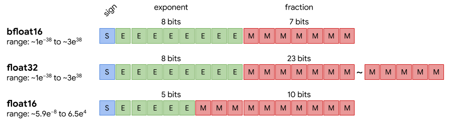
Figure 3.1: Value representation range comparison between float32, float16 and bfloat16.

3.9.1 Fundamentals of Numerical Types

3.9.2 Floating-Point Formats

A floating-point (FP) number is a way to represent real numbers in binary format (IEEE Standards Association 2019; Goldberg 1991), allowing a computer to store both very large and very small values efficiently.

It’s called floating because the radix point (the binary equivalent of the decimal point) “floats” — it can move depending on the exponent.

A floating-point number includes the following components:

Sign bit (S): determines the sign of the real number, with $0$ for positive and $1$ for negative.
Exponent bits (E): A $k$-bit field storing the exponent in biased form. The value of E stored in memory is a raw unsigned integer in range $[0, 2^k-1]$. The actual exponent used in calculations is derived by subtracting a bias from the stored exponent. The bias is a constant depending exclusively on the numerical format, hence it does not impact the number of bits required to store a number in memory.
Fraction or Mantissa bits (M): represent the precision of the number, i.e. the significant digits held after the radix point.

The equation that binds all that together:

\[\text{value} = (-1)^S \times (1 + M) \times 2^{(E - \text{bias})}\]

For instance, in the FP32 format utilizes $k=8$ bits, the range of the raw exponent is $[0, 255]$. Subtracting the bias $2^7-1 = 127$ results in the range of the true exponent $[-126, 127]$. If we wanted to represent the value $0.125 = 1/8 = 2^{-3}$, our true exponent would be $E = -3$. To store this, we add the bias: $-3 + 127 = 124$. The binary float32 representation of $0.125$ therefore is:

S = $0_{2}$
E = $01111100_{2}$ (which is $124$ in base 10)
M float32 = $00000000000000000000000_{2}$
M bfloat16 = $0000000_{2}$

FP32 (Single Precision)

Historically, Floating-Point 32 (FP32) has been the standard data type for machine learning (IEEE Standards Association 2019). Each value stored in FP32 uses 32 bits (4 bytes) of memory. Its key strengths are numerical stability, a wide dynamic range, and broad support across virtually all CPUs, GPUs, and ML frameworks.

While 4 bytes per parameter may seem reasonable, the memory demand becomes substantial as models grow. For instance, storing a 7 billion parameter model (7B) entirely in FP32 would require:

\[7 \times 10^{9} \text{ parameters} \times 4 \text{ bytes/parameter} = 28 \times 10^{9} \text{ bytes} \approx 28\,\text{GB}\]

This size highlights why multi-GPU setups are necessary for training and inference with large models in FP32. High-end NVIDIA GPUs (e.g., A100, V100), CPUs, and most training frameworks support FP32 natively, making it reliable but often less efficient compared to lower-precision formats.

FP16 (Half Precision)

Floating-Point 16 (FP16) uses 16 bits (2 bytes) per value, halving memory usage and increasing throughput—especially on modern GPUs like NVIDIA’s Ampere (A100), Volta (V100), and RTX series—which offer Tensor Cores optimized for FP16 operations (NVIDIA 2020b).

The trade-off is a smaller numerical range and lower precision, which makes FP16 prone to issues like underflow/overflow. This can especially affect small values such as gradients during backpropagation. For example, gradients smaller than FP16’s smallest representable subnormal value, about $5.96 \times 10^{-8}$, may be rounded to zero, disrupting training.

To mitigate this, mixed-precision training techniques (e.g. loss scaling, see below) are employed. In this approach, the model may use FP16 for most computations while keeping sensitive parts (e.g. weight updates) in FP32.

BF16 (Brain Floating Point 16)

bfloat16 (BF16) is a 16-bit floating-point format developed by Google (Google Cloud 2019), primarily for use in TPUs (Tensor Processing Units), though newer Intel CPUs (like Cooper Lake and Sapphire Rapids), and some GPUs (like NVIDIA A100 and H100) also support it.

BF16 retains the same 8-bit exponent as FP32, which gives it a similar dynamic range—an advantage over FP16. However, it only uses 7 bits for the mantissa, resulting in lower precision. This makes it more numerically robust than FP16, especially for training deep learning models, while still offering memory savings and speed gains.

Because BF16 avoids many of FP16’s issues with underflow and overflow, it’s becoming increasingly popular for both training and inference, particularly on TPUs and modern GPU accelerators that natively support it.

TF32 (Tensor Float-32)

TensorFloat-32 (TF32) is not a storage format but a compute optimization mode for NVIDIA Tensor Cores on Ampere+ GPUs (NVIDIA 2020a, 2020b). Unlike FP16 or BF16, tensors remain stored in full FP32 format. During matrix multiplication, Tensor Cores dynamically use TF32 precision (10-bit mantissa, 8-bit exponent) for speed, while accumulating results in full FP32 for accuracy.

This preserves FP32’s wide dynamic range (thanks to the 8-bit exponent) while reducing significand precision to speed up tensor operations—often with negligible model accuracy impact. Most frameworks (e.g., PyTorch, TensorFlow) enable TF32 on Ampere by default for GEMMs/convolutions, and you can disable it when strict FP32 numerics are required.

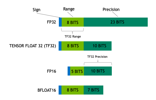
Figure 3.2: TF32 precision in comparison to FP32, FP16 and BF16.

FP8 (8-bit Floating Point)

FP8 denotes 8-bit floating‑point formats (E4M3 and E5M2) available on recent accelerators (Micikevicius et al. 2022; NVIDIA 2022). They cut memory traffic and boost matrix multiplication throughput compared to FP16/BF16.

E4M3 stands for 4 bits for exponent and 3 bits for mantissa, offers more precision but a smaller range (often used for activations/weights)
E5M2 stands for 5 bits for exponent and 2 bits for mantissa, widens the range at the cost of precision (often used for gradients).

In practice, tensors are scaled to fit the narrower FP8 range (per‑tensor or per‑channel), multiplied in FP8, and accumulated in higher precision (BF16/FP32). Master weights usually remain in FP16/BF16 or FP32 and are cast to FP8 for compute. This enables larger batches/sequence lengths and faster training/inference, provided sensitive ops (e.g., layer norm, softmax, reductions) stay in higher precision and you monitor for saturation.

Notice that successful FP8 training requires careful scaling and calibration to maintain numerical stability. Its effectiveness depends heavily on hardware support (e.g., NVIDIA Hopper+ GPUs with native FP8 Tensor Cores) and framework-specific optimizations (e.g., NVIDIA Transformer Engine). Rigorous numerical monitoring is essential to detect precision issues, and it is generally recommended to compare with higher precision formats before moving to FP8 for production workloads.

3.9.3 Integer Data Types (for Inference and Quantization)

INT8 (8-bit Integer)

INT8 is the most widely adopted quantization format today. It stores weights and activations as 8-bit integers, reducing memory by $4\times$ compared to FP32. It is supported by many hardware accelerators, including NVIDIA GPUs (TensorRT), Intel CPUs (AVX512 VNNI), Apple Neural Engine, Qualcomm Hexagon DSPs, and Google Edge TPUs.

INT8 quantization is typically used for inference, not training. It works best with post-training quantization or quantization-aware training (QAT) to minimize accuracy loss. Well-optimized INT8 models can deliver significant speed-ups ($2–4\times$) with near-FP32 accuracy on supported hardware.

INT4 (4-bit Integer)

INT4 cuts the memory in half again compared to INT8, using only 4 bits per value. It is more aggressive and can lead to greater loss in model accuracy if not handled carefully. INT4 is gaining traction with LLM quantization, especially when using weight-only quantization (not activations). Methods like GPTQ (Frantar et al. 2023), AWQ (Lin et al. 2023) allow models like LLaMA and Mistral to be quantized down to INT4 for efficient deployment on consumer GPUs (e.g., RTX 30/40 series) or edge devices.

INT4 inference is ideal when memory is limited and some loss in accuracy is acceptable in exchange for better performance and deployability.

INT1 (1-bit or Binary Neural Networks):

INT1 (or binary quantization) represents weights/activations using just 1 bit (0 or 1), providing extreme compression (up to $32\times$ smaller than FP32). This format is mainly used in Binary Neural Networks (BNNs) for highly constrained environments, such as embedded systems, IoT devices, or custom ASICs. INT1 models offer high speed and efficiency but significant accuracy trade-offs, making them unsuitable for most modern deep learning tasks unless carefully designed.

\[ \begin{array}{|l|l|l|l|l|} \hline \text{Data Type} & \text{Bit Size} & \text{Main Advantage} & \text{Typical Use Case} & \text{Hardware Support} \\ \hline \text{FP32} & \text{32-bit} & \text{High precision, wide range} & \text{Training and inference} & \text{Universal (CPUs, GPUs, TPUs)} \\ \hline \text{FP16} & \text{16-bit} & \text{Fast compute, less memory} & \text{Training (mixed-precision)} & \text{NVIDIA Tensor Cores, GPUs} \\ \hline \text{BF16} & \text{16-bit} & \text{FP32-like range, better stability than FP16} & \text{Training (mixed-precision)} & \text{TPUs, Intel CPUs, NVIDIA A100+} \\ \hline \text{TF32} & \text{32-bit} & \text{FP32-like range, faster compute} & \text{Training on NVIDIA GPUs} & \text{NVIDIA Ampere+ GPUs} \\ \hline \text{INT8} & \text{8-bit} & \text{4x smaller than FP32, fast inference} & \text{Inference} & \text{CPUs, GPUs, Edge TPUs, DSPs} \\ \hline \text{INT4} & \text{4-bit} & \text{8x smaller than FP32, extreme compression} & \text{Inference (LLMs, edge AI)} & \text{Some GPUs, ML accelerators} \\ \hline \text{INT1} & \text{1-bit} & \text{Max compression and speed} & \text{Highly constrained inference} & \text{Custom ASICs, microcontrollers} \\ \hline \end{array} \]

Table 2.5.1: Summary table of FP and INT data precision and types for training and inference.

3.9.4 Mixed Precision

In the world of modern machine learning, efficiency is just as important as accuracy. As models grow larger and more complex—especially deep neural networks with billions of parameters—the compute and memory demands skyrocket. Mixed precision techniques address this challenge by combining different numerical precisions during training and inference.

At its core, mixed precision uses both 16-bit and 32-bit floating‑point formats (for example, FP16 and FP32, or variations like bfloat16) to balance speed and stability. Computationally heavy operations (e.g., matrix multiplications and convolutions) are performed in lower precision, reducing memory usage and accelerating execution. Critical parts like weight updates and gradients remain in higher precision to preserve numerical accuracy (Yun et al. 2025; NVIDIA 2024b).

Why Mixed Precision Matters

Faster training and inference: On NVIDIA GPUs with Tensor Cores, FP16 arithmetic can be several times faster than FP32, especially in compute‑bound layers, significantly improving throughput. Compared to FP32, A100 GPUs can achieve up to $3\times$ speedups with automatic mixed precision, and V100 GPUs can see up to $8\times$ gains on certain workloads (NVIDIA 2024a).
Lower memory footprint: Since 16‑bit floats use half the storage of 32‑bit, mixed precision training reduces peak memory needs. This enables larger batch sizes or models that wouldn’t otherwise fit in GPU memory.
Broader usability: Memory efficiency allows experimentation with larger networks and faster experimental iteration which would be impractical with FP32 alone.

How Mixed Precision Works in Training

Three key techniques make mixed precision both effective and reliable:

Automatic Casting (Autocasting)
Critical math operations are automatically executed in lower precision (FP16 or BF16), while the rest remain in FP32. In more detail:
- Forward Pass: Model’s activations and inputs are computed using lower precision, usually FP16. This reduces memory usage and speeds up computations.
- Backward Pass: Gradients can be calculated in lower precision. However, they are cast (up-converted) to FP32 when updating weights to avoid underflows or overflows.
- Weights: Weights, or master weights, are maintained in memory in FP32 for accuracy and stability. During the forward pass they are downcast to lower precision. When updated, during backpropagation, they are kept in their original FP32 precision.
Loss Scaling
To avoid numerical underflow during backpropagation in low-precision, the computed loss is scaled up by a constant factor before gradient calculation, and later scaled down. This helps maintaining the gradient magnitude in a representable range while making the outcome accuracy comparable to single and double precision (Zhao et al. 2019).

\[ \begin{array}{|l|l|l|} \hline \text{Step} & \text{Operation} & \text{Precision} \\ \hline \text{1} & \text{Store model parameters} & \text{FP32 (master weights)} \\ \text{2} & \text{Cast weights for forward pass} & \text{FP16} \\ \text{3} & \text{Compute activations, losses, and gradients} & \text{FP16} \\ \text{4} & \text{Scale loss (to avoid underflow)} & \text{FP16 scaled} \\ \text{5} & \text{Unscale gradients} & \text{Convert back to FP32} \\ \text{6} & \text{Update weights using optimizer} & \text{FP32} \\ \text{7} & \text{Copy updated weights to FP16 for next iteration} & \text{FP16} \\ \hline \end{array} \]

Table 2.5.2: Mixed Precision data type conversion steps.

Why is Loss Scaling necessary for FP16-FP32 Mixed Precision?

As seen clearly in Figure 3.1, FP16 precision data types have a much smaller value representation dynamic range of $(6.1\times10^{-5}, 6.5\times10^4)$ when compared to FP32’s $(~10^{-38} , 10^{38})$. This can cause underflow or overflow when backpropagating the training loss to update our model’s weights.

In the case of gradients’ calculation, based on the loss, underflow is the risk we want to mitigate. Assuming that our gradients are FP32, or will be converted to FP32 from FP16 to update the weights, we need to effectively multiply our loss by a scale factor $f$. This serves the purpose of avoiding zeroing out very small gradients: values below FP16’s smallest normal magnitude (~$6.1 \times 10^{-5}$) fall into the subnormal range and lose precision, while those below its smallest representable value (~$5.96 \times 10^{-8}$) underflow to zero entirely. If the loss is not scaled, then we risk skipping the update of a significant number of weights. After calculating the scaled gradients, they are unscaled by a factor $1/f$ before using them to update weights.

Is Loss Scaling necessary if BF16 is used instead of FP16?

In short, loss scaling is redundant in this case. As seen in Figure 3.1, BF16 has the same dynamic range of representable values as FP32. So, it does not pose the risk of underflow, like FP16.

Mixed precision training code examples

PyTorch (PyTorch Contributors 2024)

import torch
import torch.nn as nn
import torch.optim as optim
from torch.amp import autocast, GradScaler

# Example model definition
class Net(nn.Module):
    def __init__(self):
        super(Net, self).__init__()
        self.fc = nn.Linear(10, 1)

    def forward(self, x):
        return self.fc(x)

# Creates model and optimizer in default precision
model = Net().cuda()
optimizer = optim.SGD(model.parameters(), lr=0.01)

# Creates a GradScaler once at the beginning of training.
scaler = GradScaler('cuda')

# Example loss function and dummy data
loss_fn = nn.MSELoss()
epochs = range(2)
data = [(torch.randn(16, 10, device='cuda'), torch.randn(16, 1, device='cuda')) for _ in range(10)]

for epoch in epochs:
    for input, target in data:
        optimizer.zero_grad()

        # Runs the forward pass with autocasting.
        with autocast(device_type='cuda', dtype=torch.float16):
            output = model(input)
            loss = loss_fn(output, target)

        # Scales loss and backpropagates
        scaler.scale(loss).backward()

        # scaler.step() first unscales the gradients of the optimizer's assigned params.
        scaler.step(optimizer)

        # Updates the scale for next iteration.
        scaler.update()

TensorFlow (TensorFlow Contributors 2024)

import tensorflow as tf
from tensorflow import keras
from tensorflow.keras import layers, mixed_precision

policy = mixed_precision.Policy('mixed_float16')
mixed_precision.set_global_policy(policy)

print('Compute dtype: %s' % policy.compute_dtype)
print('Variable dtype: %s' % policy.variable_dtype)

# Build Tensorflow model
# Each layer has its own default precision policy, but will use the global set
# ‘mixed_float16’. Meaning, keep variables at fp32, but do calculations in fp16
inputs = keras.Input(shape=(784,), name='digits')

if tf.config.list_physical_devices('GPU'):
  print('The model will run with 4096 units on a GPU')
  num_units = 4096
else:
  # Use fewer units on CPUs so the model finishes in a reasonable amount of time
  print('The model will run with 64 units on a CPU')
  num_units = 64
dense1 = layers.Dense(num_units, activation='relu', name='dense_1')
x = dense1(inputs)
dense2 = layers.Dense(num_units, activation='relu', name='dense_2')
x = dense2(x)

# We want the output of our model to be in fp32 for accuracy
x = layers.Dense(10, name='dense_logits')(x)
outputs = layers.Activation('softmax', dtype='float32', name='predictions')(x)
print('Outputs dtype: %s' % outputs.dtype.name) 

model = keras.Model(inputs=inputs, outputs=outputs)

# Load data and convert from uint8 to fp32 (input preprocessing happens on CPU,
# where fp32 calculations are more efficient)
(x_train, y_train), (x_test, y_test) = keras.datasets.mnist.load_data()
x_train = x_train.reshape(60000, 784).astype('float32') / 255
x_test = x_test.reshape(10000, 784).astype('float32') / 255

history = model.fit(x_train, y_train,
                    batch_size=8192,
                    epochs=5,
                    validation_split=0.2)
test_scores = model.evaluate(x_test, y_test, verbose=2)
print('Test loss:', test_scores[0])
print('Test accuracy:', test_scores[1])

3.9.5 When to use full precision

Mixed precision training has become the standard for accelerating deep learning workloads. By combining reduced-precision arithmetic (such as FP16 or BF16) with 32-bit accumulation, it delivers dramatic gains in throughput and memory efficiency — often with negligible loss in accuracy.

However, despite its appeal, mixed precision is not a one-size-fits-all solution. Certain models, algorithms, and scenarios still demand full precision (FP32) to maintain numerical stability and correct gradient flow. This section explores why and when full precision remains necessary, and how to strategically employ it alongside mixed precision for reliable model training.

Numerical precision determines how finely a floating-point number can represent real values:

FP32 (full precision) provides a 23-bit mantissa and 8-bit exponent — offering both high resolution and a wide dynamic range.
FP16 halves this, limiting dynamic range and resolution.
BF16 preserves FP32’s exponent width but truncates the mantissa.

While mixed precision training cleverly mitigates many precision-related issues, it cannot eliminate them entirely. Some computations inherently require more numerical fidelity than reduced formats can offer. In such cases, reverting to full precision is the most reliable way to ensure convergence and reproducibility.

Why and when is full-precision still relevant?

Numerical Sensitivity and Gradient Stability

Certain models — particularly those with sharp loss surfaces, delicate optimization landscapes, or extreme activation ranges — are highly sensitive to rounding error. Examples include:

Generative Adversarial Networks (GANs)
Reinforcement Learning (RL) agents with value/policy gradients
Physics-informed or differential equation-based networks
Models trained with very small batch sizes or irregular updates

In these cases, small numerical discrepancies can amplify across iterations, leading to instability or divergence. Full precision ensures gradients are faithfully represented, preserving the optimizer’s ability to make accurate updates.

Early Development and Debugging

When developing a new model or experimenting with a novel architecture, full precision provides cleaner diagnostics. Because reduced precision can mask numerical issues, debugging in FP32 ensures that observed instability stems from the model design, not arithmetic artifacts. Once the model demonstrates stable convergence, mixed precision can be reintroduced for efficiency.

Small-Scale or Memory-Rich Training

On smaller models or high-memory hardware, the computational benefit of mixed precision may be marginal. Furthermore, if the training comfortably fits in memory and meets runtime requirements, using full precision simplifies implementation and avoids the added complexity of scaling and casting between precisions.

3.9.6 Key Takeaways

Hardware trends continue to blur the boundaries between precisions. Formats like BF16 and FP8 expand the viable range for mixed-precision training, while adaptive scaling algorithms reduce underflow risks.

Nevertheless, full precision remains the gold standard for correctness and stability. Every successful mixed-precision system is anchored by a full-precision backbone — whether in master weights, accumulators, or validation loops.

Full precision (FP32) is indispensable for numerical robustness, debugging, and scientific fidelity.
Use FP32 for normalization layers, loss computation, and sensitive models or tasks.
Mixed precision should be the default for production-scale models, but always validated against a full-precision baseline.
Many efficient systems combine both — leveraging FP16/BF16 speed while retaining FP32 precision where it matters.

In essence, mixed precision accelerates deep learning, but full precision anchors it in reliability. The art of modern training lies not in choosing between the two, but in balancing them to suit the systems and models at hand.

3.10 Checkpointing and State Management

Efficient checkpointing and careful state management are critical for long-running, large-scale LLM training jobs on EuroHPC infrastructures. Unlike cloud environments where instances run indefinitely, HPC jobs often face strict wall-time limits (e.g., 24 or 48 hours), requiring jobs to stop and resume multiple times to complete training.

Furthermore, with hundreds of GPUs writing to a shared filesystem simultaneously, poor I/O patterns rarely crash the filesystem outright—but they routinely cause severe metadata contention and I/O congestion that degrade storage performance for every user on the cluster, not just your own job (George et al. 2025; NERSC 2024). This chapter focuses on when to checkpoint, how to manage distributed state efficiently, and how to avoid overwhelming HPC storage systems.

3.10.1 Checkpoint Frequency

Checkpointing is a trade-off between fault tolerance (minimizing lost work) and training throughput (minimizing time spent waiting for I/O).

General Guidelines

On EuroHPC systems, the cost of writing to disk can be high.

Frequency: For massive models, saving every few hours is standard. For smaller models or fine-tuning, saving every epoch is acceptable.
Adaptive Policies: Models are most likely to diverge in the first few thousand steps. It is wise to checkpoint frequently at the start, then reduce frequency as stability improves.
Wall-clock Limits: Always trigger a checkpoint shortly before your job’s wall-time limit expires (e.g., via a signal handler).

Example: Step-based Checkpoint Scheduling

Hard-coding a step interval is often insufficient because training speed varies. A logic that considers training phases is more robust.

def should_checkpoint(step, steps_per_hour, unstable_phase_steps):
    """
    Determines if a checkpoint is needed based on training stability and time.
    """
    # Phase 1: High instability risk. Save frequently (e.g., every 30 mins).
    if step < unstable_phase_steps:
        return step % (steps_per_hour // 2) == 0
    
    # Phase 2: Stable training. Save hourly to maximize throughput.
    else:
        return step % steps_per_hour == 0

# Example usage inside the training loop
if should_checkpoint(step, steps_per_hour=1000, unstable_phase_steps=5000):
    save_checkpoint(...)

Measuring Checkpoint Overhead

If saving a checkpoint takes 10 minutes and you do it every 20 minutes, you are wasting 50% of your GPU allocation. You must measure this overhead.

import time

start = time.time()
# The barrier ensures we measure the time for the slowest rank to finish writing
if dist.is_initialized():
    dist.barrier()
    
save_checkpoint(path, model, optimizer, scheduler, step)

# Barrier again to ensure all writes are done before timing stops
if dist.is_initialized():
    dist.barrier()
    
ckpt_time = time.time() - start

if dist.get_rank() == 0:
    print(f"Checkpoint I/O time: {ckpt_time:.2f}s")

Best practice: Treat checkpoint overhead as a budget to manage rather than a fixed limit. As a rule of thumb, overhead above ~5% of total runtime is worth investigating—but the acceptable figure depends on your context: model scale and checkpoint size, the job’s wall-time limit, the performance of the underlying filesystem, and how much progress you can afford to lose on failure. A job on a flaky partition with a short wall-time may rationally accept higher overhead to checkpoint more often, while a stable, long-allocation run should drive it lower. If overhead is high and the work-loss risk is low, reduce frequency or optimize the I/O backend (e.g., sharded or asynchronous writes, discussed below) (PyTorch Contributors 2023e; Microsoft 2024).

3.10.2 Shard Management for Distributed Training

For Large Language Models, gathering full model weights onto a single rank (Rank 0) for saving is impractical—for sufficiently large models it will cause Out-Of-Memory (OOM) errors and network congestion. Sharded checkpointing is mandatory.

Key Principles

Distributed Writes: Each GPU (or node) writes only its portion of the model and optimizer state to disk.
Metadata: A small file tracks how these shards fit together, allowing you to reload the model later even if you change the number of GPUs (topology agnostic). In practice this is not automatic for every setup: restoring at a different world size may require the framework to reshard the saved tensors, and success depends on the sharding strategy, how optimizer state is stored, and the parallelism configuration. DCP handles this for FSDP, but other parallelism schemes (e.g., tensor or pipeline parallelism) may need framework-specific handling (PyTorch Contributors 2023b, 2023e).
Format: Use modern formats like PyTorch DistributedCheckpoint (DCP) (PyTorch Contributors 2023e) over legacy torch.save-based methods.

Example: PyTorch FSDP Distributed Checkpoint

When using Fully Sharded Data Parallel (FSDP) (PyTorch Contributors 2023c), the model weights are already split across GPUs. Saving them directly in this sharded state is highly efficient.

import torch.distributed.checkpoint as dcp
from torch.distributed.checkpoint.state_dict import get_state_dict

# Retrieve the (sharded) model and optimizer state dicts. With FSDP each rank
# holds only its own shard, so this stays memory-efficient.
model_state, optim_state = get_state_dict(fsdp_model, optimizer)
state_dict = {"model": model_state, "optimizer": optim_state}

# Writes directly to a directory using efficient parallel I/O
dcp.save(
    state_dict=state_dict,
    storage_writer=dcp.FileSystemWriter("/mnt/lustre/project_x/fsdp_ckpt_step_1000"),
)

Example: Loading a Sharded Checkpoint

Loading is the reverse process. DCP handles the complexity of mapping shards on disk to the current GPU topology.

from torch.distributed.checkpoint.state_dict import get_state_dict, set_state_dict

# Build template state dicts that DCP will populate in place.
model_state, optim_state = get_state_dict(fsdp_model, optimizer)
state_dict = {"model": model_state, "optimizer": optim_state}

# DCP maps the on-disk shards onto the current GPU topology.
dcp.load(
    state_dict=state_dict,
    storage_reader=dcp.FileSystemReader("/mnt/lustre/project_x/fsdp_ckpt_step_1000"),
)

# Apply the loaded tensors back to the model and optimizer.
set_state_dict(
    fsdp_model,
    optimizer,
    model_state_dict=model_state,
    optim_state_dict=optim_state,
)

Best practice: Validate that sharded checkpoints can be restored with a different world size before you rely on it—do not assume it works for free. This allows you to continue training even if fewer nodes are available in your next allocation, but because changing world size can trigger resharding and depends on framework support, the only reliable confirmation is an actual reload-and-resume test at the target GPU count.

Asynchronous Checkpointing

The overhead measured earlier comes largely from GPUs sitting idle while the slowest rank finishes writing to disk. Asynchronous checkpointing hides most of that cost by splitting the save into two phases: a fast, blocking staging step that snapshots the state (typically copying tensors from GPU into pinned CPU memory), followed by a background write to the filesystem that overlaps with subsequent training steps. The GPUs resume computing as soon as staging finishes, so the wall-clock penalty drops from “time to write the whole checkpoint” to “time to copy it to host memory.”

PyTorch DCP exposes this through dcp.async_save, which returns a future while a background thread performs the I/O (PyTorch Contributors 2023e).

import torch.distributed.checkpoint as dcp

checkpoint_future = None

def save_async(state_dict, path):
    global checkpoint_future
    # Ensure the previous checkpoint has finished writing before staging a new one.
    if checkpoint_future is not None:
        checkpoint_future.result()
    # Returns once staging is done; the disk write proceeds in the background.
    checkpoint_future = dcp.async_save(
        state_dict=state_dict,
        storage_writer=dcp.FileSystemWriter(path),
    )

Key caveats:

Staging is not free. It still blocks briefly and needs spare host memory to hold a snapshot of model and optimizer state—budget for the extra RAM.
Join the outstanding future before the next save and before the job exits; otherwise an abrupt termination can leave a half-written checkpoint on disk.
Treat the most recent async checkpoint as in-flight until its write completes—your “latest valid checkpoint” for resume purposes is the last one whose future returned successfully.

DeepSpeed offers equivalent functionality through its asynchronous and NVMe-offloaded checkpointing paths (Microsoft 2024).

Best practice: On bandwidth-constrained shared filesystems, asynchronous checkpointing is often the single most effective way to raise checkpoint frequency without paying for it in GPU idle time.

3.10.3 Redundancy and Reliability

A checkpoint file is a valuable scientific artifact. On high-performance parallel file systems (like Lustre or GPFS), file corruption or silent write failures can happen.

Storage Strategy

Tier 1 (Fast/Scratch): Use the high-speed parallel filesystem (e.g., /scratch or /lustre) for active checkpointing.
Tier 2 (Work): Move critical milestones to persistent project storage.
Tier 3 (Backup): For “gold” checkpoints (final models), copy to object storage or a different facility.

Checksum Verification

Never assume a write was successful just because no error was thrown. Generate checksums to detect “bit rot.”

# Generate SHA256 checksum immediately after saving
sha256sum checkpoint.pt > checkpoint.pt.sha256

# Verify before loading to prevent crashing with obscure errors
sha256sum -c checkpoint.pt.sha256

Periodic Recovery Testing

A common horror story involves training for weeks, only to find the checkpoints are incompatible with the loading script.

# Run a dummy job that loads the latest checkpoint and runs 10 steps
python train.py --resume /path/to/checkpoint.pt --max_steps 10

This verifies that the checkpoint is:

Readable (filesystem accessible)
Complete (no missing keys)
Compatible (codebase hasn’t drifted)

Best practice: Automate a “canary” job that attempts to load the checkpoint immediately after it is saved.

3.10.4 Storage Policies

LLM checkpoints are massive. A 70B parameter model with optimizer states can exceed 500 GB per checkpoint. Storing thousands of steps will fill your group’s quota and annoy HPC administrators.

Retention Policies

Rolling Window: Keep only the last 3-5 checkpoints for immediate resume capabilities.
Milestones: “Pin” checkpoints that represent significant progress (e.g., end of an epoch, best validation loss).
Cleanup: Automate the deletion of intermediate checkpoints.

Example: Automatic Pruning Script

Do not rely on manual cleanup. Integrate pruning into your training loop or a separate cron job.

import os
import glob

def prune_checkpoints(ckpt_dir, keep_last=5):
    # Find all checkpoints matching the pattern
    ckpts = sorted(glob.glob(os.path.join(ckpt_dir, "ckpt_step_*.pt")))
    
    # Identify which ones are old
    to_delete = ckpts[:-keep_last]
    
    for path in to_delete:
        try:
            # If it's a directory (sharded ckpt), use shutil.rmtree
            # If it's a file, use os.remove
            if os.path.isdir(path):
                import shutil
                shutil.rmtree(path)
            else:
                os.remove(path)
            print(f"Deleted old checkpoint to free space: {path}")
        except OSError as e:
            print(f"Error deleting {path}: {e}")

# Call this after a successful save
prune_checkpoints("./checkpoints", keep_last=5)

I/O-Aware Scheduling

Parallel filesystems perform best with large, sequential writes.

Avoid: Thousands of tiny files (e.g., one file per tensor per GPU).
Prefer: Consolidated binary blobs (standard in torch.distributed.checkpoint).

Best practice: Treat storage as a shared finite resource. If you fill the filesystem, you block not just your team, but every user on the supercomputer.

3.10.5 State Consistency and Completeness

A common mistake is saving the model weights but forgetting the auxiliary state. If you lose the optimizer state (momentum), the model effectively “forgets” the direction it was traveling, causing a massive loss spike upon resumption.

Ensure the Following Are Saved

checkpoint = {
    # 1. The Weights
    "model": model.state_dict(),
    
    # 2. The Learning Trajectory (Momentum, Variance)
    "optimizer": optimizer.state_dict(),
    
    # 3. The Learning Rate Schedule
    "scheduler": scheduler.state_dict(),
    
    # 4. FP16/BF16 Scaling Factors (Crucial to prevent underflow on resume)
    "scaler": scaler.state_dict() if use_amp else None,
    
    # 5. Global Step Count
    "step": step,
    
    # 6. Random Number Generator States (Ensures data shuffling order persists)
    "rng_cpu": torch.get_rng_state(),
    "rng_cuda": torch.cuda.get_rng_state_all(),
}

# Save strictly consistent state
torch.save(checkpoint, path)

Best practice: After resuming, explicitly log the loss and learning rate for the first 10 steps. They should closely match the trajectory of the previous run (bitwise-identical values are not guaranteed across different hardware or library versions). If the loss spikes, you are likely missing optimizer or scaler state.

By combining adaptive checkpoint frequency, efficient sharded state management, redundancy mechanisms, and strict storage policies, researchers can ensure robust state preservation and rapid recovery.

Well-designed checkpointing is not just a safety feature—it is the mechanism that allows massive, multi-week training jobs to survive the realities of shared EuroHPC infrastructure.

3.11 Evaluation and Model Monitoring

Accurately measuring the capabilities of LLMs both during and after training is crucial for understanding their strengths and weaknesses. A strong evaluation framework allows researchers to track progress, identify areas for improvement, and make informed decisions about future development and deployment. It also allows one to detect biases, ensure fairness, and assess the real-world applicability of these models—not to mention the importance of detecting catastrophic forgetting and other issues that may arise during training.

This pressing need has led to the development of a vibrant and active research field focused on creating robust evaluation frameworks and benchmarks for LLMs. In this section, we are going to discuss some of the most widely used benchmarks and evaluation frameworks for LLMs, highlighting their strengths and limitations.

3.11.1 Train-Time Monitoring

Monitoring model performance during training is essential to ensure that the model is learning effectively and to identify potential issues early on. A ubiquitous practice when training LLMs is to split data into training, validation, and test data. The training data is used to update the model’s weights, while the validation data is used to monitor the model’s performance during training. The test data is used to evaluate the model’s performance after training is complete.

In practice, modern LLM training pipelines go well beyond a single validation/test split. It is common to maintain multiple complementary validation sets, each targeting a different domain or capability (e.g., code, mathematical reasoning, multilingual text), alongside continual benchmark tracking against established suites such as HELM (Liang et al. 2023). This multi-faceted approach helps detect regressions in specific capabilities that a single aggregate validation loss might mask. Periodic evaluations on external benchmarks further ensure that improvements on one axis do not come at the cost of degradation on another. In smaller-scale or research settings, cross-validation can also be a valuable strategy—rotating which portion of the data serves as the validation set—to obtain more robust estimates of model performance and reduce sensitivity to any particular data split. However, due to the computational cost, cross-validation is rarely practical for full-scale LLM pretraining and is more commonly applied during fine-tuning or ablation studies. Scaling laws research (Kaplan et al. 2020) has also shown that systematic evaluation across multiple data scales and model sizes can inform decisions about when and how to evaluate during training.

When monitoring model performance during training, there are several key aspects to consider:

Training Loss: Tracking the training loss over time provides insights into how well the model is learning from the training data. A decreasing training loss indicates that the model is improving its ability to fit the training data.
Validation Loss: Monitoring the validation loss helps to assess the model’s generalization capabilities. If the validation loss starts to increase while the training loss continues to decrease, it may indicate overfitting.
Gradient Norms: Monitoring the norms of gradients can help to identify issues such as exploding or vanishing gradients, which can hinder the training process.
Learning Rate Schedules: Tracking the learning rate and its adjustments during training provides insights into the optimization process and can help to identify potential issues with convergence, also when compared to the training and validation loss curves.
Weights Norms: Monitoring the norms of the model’s weights can help to identify potential issues such as exploding weights, which can lead to instability during training.
Throughput and Latency: Tracking the training throughput (e.g., tokens per second) and latency can help to identify potential bottlenecks in the training process and optimize resource utilization.
Custom Metrics: Depending on the specific task and model architecture, it may be beneficial to monitor custom metrics that are relevant to the model’s performance, such as accuracy, F1 score, or perplexity.

It is also possible to perform occasional evaluations on a subset of the test data during training to get a sense of how the model will perform once training is complete. However, to avoid overfitting to the test data, it is important to limit this practice to a small number of samples or benchmarks. Otherwise, any overfitting of the benchmarks will not be detected at the end of training.

Loss Spikes and Instability Detection

During large-scale training runs, practitioners may encounter sudden disruptions in the training process that manifest as loss spikes—abrupt, large increases in training loss that deviate sharply from the expected downward trend. In severe cases, the loss may diverge to NaN, halting training entirely. Gradient norm explosions, where gradient magnitudes jump by several orders of magnitude, often accompany or precede these events.

Loss spikes typically arise from one or more of the following causes:

Bad data batches: Corrupted, degenerate, or anomalously long samples in the training data can produce extreme gradient updates. Data quality issues that only affect a small fraction of the corpus may go unnoticed during preprocessing but surface during training.
Learning rate misconfiguration: A learning rate that is too high—or a warmup schedule that ramps up too aggressively—can push the model into unstable regions of the loss landscape.
Numerical overflow in mixed precision: When training with reduced-precision formats, intermediate activations or gradients may exceed the representable range, producing infinities or NaN values that propagate through the computation graph. The severity differs between formats: FP16 (5 exponent bits, max ~65,504) is prone to overflow and typically requires loss scaling, whereas BF16 (8 exponent bits, max ~3.4×10³⁸) largely eliminates overflow concerns thanks to its FP32-matching exponent (Kalamkar et al. 2019). BF16’s reduced mantissa (7 bits vs. FP16’s 10) can still introduce rounding errors that accumulate over long runs.

Effective response strategies include:

Gradient clipping: Capping gradient norms to a maximum value (a common default being 1.0) to limit the impact of any single update.
Automatic rollback: Periodically saving checkpoints and rolling back to the last healthy checkpoint when a spike is detected.
Batch skipping: Detecting and skipping batches that produce anomalously large gradient norms, preventing a single bad sample from derailing the entire run.
Learning rate reduction: Temporarily reducing the learning rate after a spike to allow the model to recover smoothly, then gradually restoring it.

Monitoring gradient norms, loss values, and weight norms (as discussed in the metrics above) is essential for early detection. Setting up automated alerts—for example, triggering when the loss exceeds a rolling average by more than a configurable threshold—can significantly reduce the time between a spike occurring and the team responding.

3.11.2 Model Monitoring Tools

There are several tools available to support practitioners in monitoring model performance during training. Some of the most popular tools include: WandB (Weights & Biases 2020), TensorBoard (Google 2019), and MLflow (Databricks 2018). These tools provide a range of features for tracking and visualizing model performance, including: automatic logging of metrics, customizable dashboards, and integration with popular deep learning frameworks.

When selecting a model monitoring tool, it is important to consider factors such as ease of use, integration with existing workflows, and support for custom metrics. Additionally, it may be beneficial to choose a tool that supports collaboration and sharing of results among team members.

For instance, WandB provides a collaborative platform that allows team members to share and discuss model performance metrics in real-time. However, it requires compute nodes to have internet access to log metrics to WandB servers (although manual upload is possible). Furthermore, WandB offers advanced features such as hyperparameter tuning and model versioning, which can be useful for managing complex training workflows.

Alternatively, TensorBoard is a widely used tool that provides a range of visualization options for tracking model performance. It is tightly integrated with TensorFlow, but can also be used with other deep learning frameworks through plugins. TensorBoard offers features such as scalar plots, histograms, and image visualizations, which can help to gain insights into the model’s learning process.

MLflow is another popular tool that provides a range of features for tracking and managing machine learning experiments. It offers a centralized platform for logging metrics, managing models, and tracking data versions. MLflow supports integration with popular deep learning frameworks and provides a range of APIs for customizing the monitoring process.

3.11.3 Evaluation Frameworks

When deciding which evaluation framework to use, it is important to account for a few key factors:

Task Diversity: The framework should cover a wide range of tasks to ensure a comprehensive evaluation of the model’s capabilities. This includes tasks such as: question answering, mathematical reasoning, code generation, and more.
Number of Benchmarks: A framework that supports the evaluation of multiple benchmarks allows for a more thorough assessment of the model’s performance. Having a variety of benchmarks for the same task often allows to have a more nuanced evaluation and understanding of the model’s behavior.
Scalability: The framework should be able to handle large-scale evaluations, especially when dealing with LLMs that require significant computational resources. For example, supporting evaluation through external APIs providers (e.g., OpenAI, Cohere, etc.) or being able to checkpoint and resume evaluations are important features to consider.
Customization: The ability to customize the evaluation process, such as: adding new benchmarks, modifying existing ones, or adjusting evaluation metrics, is important for tailoring the evaluation to specific needs.
Ease of Use: A user-friendly interface and clear documentation can significantly reduce the learning curve and make it easier for practitioners to adopt the framework.

The most widely used evaluation frameworks for LLMs include: LM Evaluation Harness, OpenCompass, and DeepEval. Each of these frameworks has its own strengths and weaknesses, and the choice of which one to use will depend on the specific needs and requirements of the user.

LM Evaluation Harness

LM Evaluation Harness (Gao et al. 2023) is an open-source library developed by EleutherAI for evaluating language models on a variety of benchmarks. It is designed to be easy to use and supports a wide range of tasks, including: text classification, question answering, and more. It is highly customizable and allows users to add their own benchmarks and evaluation metrics. It supports both local models and models accessed through APIs (e.g., OpenAI, Cohere, etc.). Support for vLLM-served models is also available, allowing scalable evaluations.

In LM Evaluation Harness, evaluations are mostly managed through a command-line interface, lm_eval. It supports a variety of arguments to customize the evaluation process, including support for vLLM models, batch size, number of GPUs, and more. A typical evaluation command looks like this:

lm_eval --model vllm \
    --model_args pretrained={model_name},tensor_parallel_size={GPUs_per_model},dtype=auto \
    --tasks {task_name} \
    --batch_size auto

More advanced usage can be achieved by creating a custom python script that uses the library’s API. This accommodates more complex evaluation scenarios, such as evaluating multiple models or tasks in a single run, or customizing the evaluation metrics.

OpenCompass

OpenCompass (Contributors 2023) is an open-source comprehensive evaluation framework for LLMs. It supports a wide range of tasks and benchmarks. It is highly customizable and scalable. However, the documentation is scarce and the learning curve is quite steep.

In OpenCompass, evaluations are organized into configuration files written in the mmengine (MMEngine Contributors 2022) style, a pure Python-based configuration system. Each configuration should specify 5 main components:

datasets: a list of datasets to be used for evaluation.
models: a list of model configurations. Each model configuration is evaluated against all the datasets specified in the datasets field. A variety of model types are already supported, including OpenAI API, HuggingFace models, and more.
infer (Optional): the inference configuration, which specifies how inference is partitioned across tasks, the number of concurrent workers, etc.
eval (Optional): the evaluation configuration, which specifies how scoring is partitioned across tasks, the number of concurrent workers, etc.
summarizer (Optional): a configuration for generating the final evaluation report.

Configurations are deployed through a command-line interface, opencompass. A typical evaluation command looks like this:

opencompass configuration.py -w outputs

For basic usages, the configuration file may be optional, as opencompass supports a variety of command-line arguments to customize the evaluation process. However, for more advanced usage, creating a configuration file is recommended.

DeepEval

DeepEval (Ip and Vongthongsri 2026) is an open-source evaluation framework developed by Confident AI. It is designed to be easy to use and supports a wide range of tasks. It is highly customizable and allows users to add their own benchmarks and evaluation metrics. It does not directly provide support for inference. However, it is fairly easy to integrate with other libraries, such as Hugging Face or vLLM, to evaluate local models.

In DeepEval, evaluations are mostly managed through a python script that uses the library’s API. A typical evaluation script looks like this:

from deepeval.benchmarks import GSM8K
benchmark = GSM8K(n_problems=10, n_shots=3)
benchmark.evaluate(model=your_model)

LightEval

LightEval (Habib et al. 2023) is an open-source evaluation framework developed by Hugging Face. It is designed to be lightweight and easy to use, with a focus on evaluating language models on a variety of benchmarks. It supports both local models and models accessed through APIs (e.g., OpenAI, Cohere, etc.). It supports a wide range of tasks. However the customization options are limited compared to other frameworks.

In LightEval, evaluations are mostly managed through a command-line interface, lighteval. It supports a variety of arguments to customize the evaluation process. A typical evaluation command looks like this:

lighteval accelerate \
    "model_name=gpt2" \
    "leaderboard|truthfulqa:mc|0"

Custom Evaluation

Several benchmarks, such as BFCL (Patil et al. 2023), come with their own evaluation scripts. In such cases, it may be more convenient to adopt directly the provided scripts, rather than using a general purpose evaluation framework.

3.11.4 Benchmark Domains

When evaluating general purpose LLMs, it is important to consider a variety of benchmark domains to ensure a comprehensive assessment of the model’s capabilities. Benchmark domains can be broadly categorized into two main types: pure text benchmarks and multimodal benchmarks. The former focuses on evaluating the model’s performance on text-based tasks, while the latter assesses the model’s ability to handle and integrate multiple modalities, such as text, images, and audio.

Pure text benchmarks:
- Mathematical Reasoning: Evaluating the model’s ability to solve mathematical problems, including arithmetic, algebra, and calculus. Examples of benchmarks in this domain include: GSM8K, MATH500, AIME24, and AIME25.
- Code Generation: Assessing the model’s ability to generate and understand code in various programming languages. Examples of benchmarks in this domain include: HumanEval, MBPP, and LiveCodeBench.
- Abstract Reasoning: Testing the model’s ability to perform abstract reasoning tasks, such as pattern recognition and logical reasoning. Examples of benchmarks in this domain include: ARC-AGI-1, ARC-AGI-2, and RAVEN.
- Instruction Following: Measuring the model’s ability to follow instructions and perform tasks based on given prompts. Examples of benchmarks in this domain include: IFeval, AlpacaEval, and Evol-Instruct.
- Scientific Knowledge: Testing the model’s understanding of scientific concepts and its ability to answer questions related to various scientific fields. Examples of benchmarks in this domain include: GPQA, PubMedQA, and SciQ.
- General Knowledge and Reasoning: Evaluating the model’s ability to answer questions and perform reasoning tasks that require a broad understanding of various topics. Examples of benchmarks in this domain include: MMLU, TruthfulQA, and OpenBookQA.
- Ethics and Bias: Assessing the model’s ability to handle ethical dilemmas and avoid biased responses. Examples of benchmarks in this domain include: ETHICS, BBQ, and BiasBench.
- Tool Use: Evaluating the model’s ability to use external tools, such as calculators or search engines, to enhance its performance on various tasks. Examples of benchmarks in this domain include: ToolBench and BFCL.
Multimodal benchmarks:
- Image Understanding: Assessing the model’s ability to understand and interpret images, including tasks such as image captioning and visual question answering. Examples of benchmarks in this domain include: VQA, COCO Captioning, and ImageNet.
- Video Understanding: Evaluating the model’s ability to analyze and interpret video content, including tasks such as action recognition and video captioning. Examples of benchmarks in this domain include: Kinetics, ActivityNet, and YouCook2.
- Audio Understanding: Measuring the model’s ability to process and understand audio content, including tasks such as speech recognition and music classification. Examples of benchmarks in this domain include: libriSpeech and AudioSet.
- Multimodal Reasoning: Testing the model’s ability to reason across multiple modalities, such as combining text and images to answer questions or perform tasks. Examples of benchmarks in this domain include: VCR, NLVR2, and MM-Vet.

3.11.5 Common Challenges in Evaluations

Task Formulation

While evaluating already trained LLMs is relatively straightforward, evaluating models in earlier stages of training (e.g., before ~1T tokens) is significantly more challenging. At that stage, generation quality may still be unstable, making certain evaluation setups noisy or unreliable. The way a task is formulated therefore plays a central role in obtaining meaningful and comparable results.

In general, two main evaluation paradigms are used:

Free-Form Generation

In free-form generation, the model is prompted to generate an unconstrained response to a question or instruction. This is the most natural setup and is widely used for instruction-following, reasoning, and coding benchmarks, including tasks in LM Evaluation Harness and standardized evaluations such as HELM.

While simple conceptually, this formulation presents several challenges:

High sensitivity to prompt wording.
Variance introduced by sampling parameters.
Difficulty in automatically extracting the final answer.
Poor reliability for very early training checkpoints.

Prompting strategies such as chain-of-thought (Wei et al. 2022) can significantly improve reasoning performance by asking the model to produce intermediate steps before the final answer. However, they also change task difficulty and must be applied consistently across models for fair comparison.

Few-shot prompting can further improve results—especially for base (non-instruction-tuned) models—but increases context length usage and may introduce additional variance.

Cloze and Multiple-Choice Formulation

In cloze-style evaluation, the model selects or scores a candidate completion rather than generating an answer from scratch. This setup is common in multiple-choice benchmarks such as MMLU.

Typically, evaluation is performed by computing the log-likelihood of each candidate answer and selecting the most probable one. Compared to free-form generation, this approach:

Reduces output variance.
Avoids complex answer parsing.
Is more suitable for early-stage models.
Enables deterministic evaluation (e.g., greedy decoding).

However, formatting details still matter. The way answer choices are presented (e.g., labeled A/B/C/D vs. inline text), the order of options, and whether reasoning is requested can all affect performance—sometimes significantly for very early checkpoints.

Identifying the answer

Identifying the LLMs answer is one of the most common challenges in evaluating LLMs. As the LLMs may provide the results in a wide variety of formats. For example, when the answer is a number, the LLM may answer with 42, the answer is 42, the answer is <answer>42</answer>, forty-two, or even the answer is \boxed{42}. This makes it difficult to automatically parse the answer and compare it to the expected result.

To address this issue, special instructions are often included in the prompt or in the system message, asking the LLM to provide the answer in a specific format. For example, a typical system prompt may look like this:

You are an helpful assistant specialized in solving mathematical problems. Provide a step-by-step solution to the problem, followed by the final answer encapsulated between <answer> and </answer> tags.

Even when such instructions are provided, it is not guaranteed that the LLM will output the answer with a consistent format. To this end, specialized parsers and evaluators are often employed to extract the answer and compare it to the expected result, see Math-Verify (Kydlíček, n.d.) for an example.

For coding tasks, the model is usually required to return its answer inside a fenced code block (for example, a Python code block delimited by triple backticks).

Evaluating Open-Ended Tasks

Open ended tasks, such as question answering may not even have a single correct answer or there may not be a straightforward way to compare the LLMs answer to the expected result. For example, consider the following question:

What are the benefits and drawbacks of using renewable energy sources?

In such cases, it is often necessary to use more sophisticated evaluation methods, such as human evaluation or using another LLM as a judge. In the latter case, the LLM is first prompted with the question and then, either the same or a different LLM is prompted to evaluate the answer provided by the first LLM against the expected result. This approach can be effective, but it relies heavily on the quality of the judge for the evaluation to be accurate and reliable.

Generation Parameters

When evaluating LLMs, it is important to consider the generation parameters used during the evaluation. Different generation parameters can lead to significantly different results. For example, using a higher temperature may lead to more diverse and creative responses, but it may also increase the likelihood of generating incorrect or nonsensical answers. Conversely, using a lower temperature may lead to more conservative and accurate responses, but it may also limit the model’s ability to generate novel or interesting answers.

Overall, the most commonly used generation parameters include:

Temperature: Controls the randomness of the model’s output. A higher temperature (e.g., 0.7) leads to more diverse and creative responses, while a lower temperature (e.g., 0.2) leads to more conservative and focused responses.
Top-p (nucleus sampling): Limits the model’s output to a subset of the most probable tokens, based on a cumulative probability threshold. For example, a top-p value of 0.9 means that the model will only consider the smallest set of tokens whose cumulative probability is at least 0.9.
Top-k: Limits the model’s output to the k most probable tokens. For example, a top-k value of 50 means that the model will only consider the 50 most probable tokens when generating its output.
Min-p: Sets a minimum probability threshold for the tokens to be considered during generation. For example, a min-p value of 0.01 means that the model will only consider tokens with a probability of at least 0.01 when generating its output.

For example, Qwen3-8B (Qwen Team 2025) suggests the following generation parameters for best results in thinking mode (which change for the non-thinking mode):

{
  "temperature": 0.6,
  "top_p": 0.95,
  "top_k": 20,
  "min_p": 0.0
}

When deciding which generation parameters to use, it may be helpful to run a small-scale grid search on a few samples to identify good candidates. Alternatively, the above are a popular choice.

Decoding Strategies

While the most common decoding strategy used when evaluating LLMs is sampling, other strategies may offer better results. For example, beam search is a popular decoding strategy that can be used to improve the quality of the generated output. Beam search works by maintaining a fixed number of the most probable sequences at each step of the generation process, and expanding them in parallel. This allows the model to explore multiple possible outputs and select the most likely one.

Another alternative is Greedy Decoding, which simply selects the most probable token at each step of the generation process. While this approach is fast and simple, it may lead to suboptimal results. When setting temperature to 0, serving libraries such as vLLM (Kwon et al. 2023) default to Greedy Decoding.

A recent alternative is DeepConf (Fu et al. 2025), a decoding strategy that maintains a set of candidate generations rejecting those with low confidence. This approach has been shown to improve the quality of the generated output.

Regardless of the decoding strategy used, it is important to ensure that the evaluation is consistent across different models and benchmarks.

Dealing with Variance

Several popular benchmarks, such as AIME24 and AIME25, have a relatively small number of problems (30 each). When evaluating LLMs on such benchmarks, it is important to account for the variance that setting sampling parameters (e.g., temperature, top_p, etc.) may introduce. For example, when using a temperature of 0.7, the LLM may provide different answers to the same question when prompted multiple times leading potentially to highly variable results. For example, the same model, with the same sampling parameters, may achieve in two different runs accuracies of 20% and 50% on the same benchmark.

To address this issue, it is common to run several generations for each problem and then aggregate the results. For example, one may run N generations per problem and average the results. Alternatively, one may consider more sophisticated aggregation methods, such as g-pass@k (Liu et al. 2025). G-pass@k generalizes pass@k by measuring the probability that at least a given proportion of k attempts are correct, capturing not only peak capability but also the model’s consistency. This metric is particularly useful for benchmarks with a small number of problems, and it should be the preferred aggregation method, although it requires considerably scaling the number of generations per problem.

Beyond aggregation, it is important to quantify the statistical uncertainty of reported scores, especially when comparing models with similar performance. On a 30-problem benchmark, a few-point accuracy difference may well fall within statistical noise. Confidence intervals—computed via bootstrap resampling over problems or generation runs—provide a principled way to assess whether observed differences are meaningful. Evaluation suites such as HELM (Liang et al. 2023) report confidence intervals alongside scores for this reason. When bootstrap estimation is impractical, even simple standard error estimates over repeated evaluation runs can help avoid over-interpreting differences that are not statistically significant.

Scaling Evaluations

Often, a comprehensive evaluation of an LLM may require collecting results from multiple benchmarks, each of which may contain a large number of problems, and each problem may require multiple generations to account for variance. Further, when benchmarking we need a few models as baselines. This leads to an exploding number of required generations.

To address this issue, scaling the number of replicas for each model can be an effective strategy to complete the benchmarks in a reasonable amount of time. Tools like vLLM (Kwon et al. 2023) and Domyn Swarm (Domyn 2025) can be used to efficiently manage and scale the evaluation process across multiple GPUs and machines.

At this scale, evaluation itself becomes a significant infrastructure workload. Pipelines can become GPU-bound when serving large models for inference, memory-bound when long context lengths or large batch sizes exhaust available VRAM, storage-bound when loading multiple checkpoints and writing generation outputs, or API-rate-limited when evaluating through external providers. Practical strategies to manage these costs include:

Scheduling evaluations off-peak: Running evaluation jobs during periods when training clusters are underutilized to avoid competing with training for GPU resources.
Result caching: Storing generation outputs so that re-scoring with a different metric or parser does not require re-running inference. Frameworks such as LM Evaluation Harness (Gao et al. 2023) support caching of model outputs for this purpose.
Distributed inference: Using tensor parallelism or pipeline parallelism via serving engines like vLLM to spread a single large model across multiple GPUs, reducing per-evaluation latency.
Selective evaluation: Not every checkpoint needs to be evaluated on every benchmark. A tiered strategy—running lightweight benchmarks frequently and expensive ones only at key milestones—can substantially reduce overall cost.

Restoring Evaluations

When evaluating LLMs on a large number of benchmarks, it is important to be able to restore evaluations in case of interruptions or failures. This is particularly important when dealing with large models that require significant computational resources and time to evaluate. To this end, it is important to either use an evaluation framework that supports checkpointing and resuming evaluations, or implement a custom solution that can save the state of the evaluation process and resume it later.

Data Contamination and Benchmark Leakage

A critical validity threat in LLM evaluation is data contamination—the presence of benchmark samples (or close paraphrases thereof) in the model’s training data. When a model has already seen test problems during training, its performance on those benchmarks is artificially inflated, leading to misleading comparisons and a false sense of the model’s true capabilities.

This problem is particularly insidious in the era of web-scale training corpora. Popular benchmarks are widely discussed online, and their problems frequently appear on forums, blogs, and educational websites. As a result, even without intentional inclusion, benchmark data may be inadvertently scraped into training sets (Jacovi et al. 2023).

Detection approaches for data contamination include:

N-gram overlap analysis: Comparing training data against benchmark samples using n-gram matching to identify exact or near-exact duplicates.
Perplexity-based detection: Contaminated samples tend to exhibit anomalously low perplexity under the trained model compared to held-out samples of similar difficulty. A significant perplexity gap between known-clean and suspected-contaminated samples can signal leakage.

Mitigation strategies include:

Decontamination pipelines: Incorporating benchmark-aware filtering during data preparation, removing training samples that have high overlap with known evaluation sets.
Dynamic and live benchmarks: Using benchmarks that are periodically refreshed with new problems, such as LiveCodeBench (Jain et al. 2024), which continuously collects new competitive programming problems. This limits the window during which contamination is possible.
Private held-out test sets: Maintaining evaluation sets that are never publicly released, ensuring they cannot be inadvertently included in training data.

It is worth noting that even partial contamination can affect results. Rephrased versions of benchmark problems, or problems that share the same reasoning structure with slightly different surface forms, can still provide the model with an unfair advantage. For this reason, contamination analysis should go beyond exact matching and consider semantic similarity as well.

3.11.6 Most Commonly Used Benchmarks

It is worth introducing some of the most commonly used benchmarks for evaluating LLMs, even if it is just to familiarize with the kinds of tasks that are typically used to assess the capabilities of these models.

AIME24 and AIME25

AIME24 (PrimeIntellect 2024) and AIME25 (PrimeIntellect 2025) are datasets consisting of problems from the 2024 and 2025 American Invitational Mathematics Examination (AIME). Both benchmarks contain 30 problems that require mathematical reasoning and problem-solving skills. The problems are designed to be challenging and cover a wide range of mathematical topics, including algebra, geometry, number theory, and combinatorics.

An example problem from AIME24 is the following:

Among the 900 residents of Aimeville, there are 195 who own a diamond ring, 367 who own a set of golf clubs, and 562 who own a garden spade. In addition, each of the 900 residents owns a bag of candy hearts. There are 437 residents who own exactly two of these things, and 234 residents who own exactly three of these things. Find the number of residents of Aimeville who own all four of these things.

GSM8K

GSM8K (Cobbe et al. 2021) (Grade School Math 8K) is a dataset consisting of 8,500 grade school-level math word problems. The problems are designed to test the model’s ability to perform mathematical reasoning and problem-solving skills. The dataset covers a wide range of mathematical topics, including arithmetic, algebra, and geometry.

An example problem from GSM8K is the following:

Weng earns $12 an hour for babysitting. Yesterday, she just did 50 minutes of babysitting. How much did she earn?

LiveCodeBench

LiveCodeBench (Jain et al. 2024) is a continuously updated dataset of coding problems (numbering in the several hundreds and growing with each release) that require the model to generate code in response to a given prompt. Problems are collected from competitive programming platforms, such as Codeforces and LeetCode, and cover a wide range of programming topics, including algorithms and data structures.

An example problem from LiveCodeBench is the following:

You are given a positive integer array `nums`. Return the total frequencies of elements in `nums` such that those elements all have the maximum frequency.

GPQA

GPQA (Rein et al. 2023) (Graduate-Level Google-Proof Q&A) is a multiple-choice dataset consisting of 448 questions written and validated by experts in various fields, including biology, physics, and chemistry. The questions are designed to test the model’s ability to answer questions that require a broad understanding of various topics.

An example problem from GPQA is the following:

In a parallel universe where a magnet can have an isolated North or South pole, Maxwell’s equations look different. But, specifically, which of those equations are different?

3.11.7 Third-Party Evaluations

Services such as Artificial Analysis (Artificial Analysis 2024) already offer a wide range of third-party evaluations for LLMs, covering the most popular benchmarks and tasks. Such services can be useful to quickly assess positioning with respect to the state of the art. Of course, when comparing with these third-party evaluations, it is important to ensure a good level of alignment in terms of generation parameters, decoding strategies, and scoring methods.