2 Infrastructure Foundations for Scalable LLM Training

2.1 Compute

This chapter presents different types of accelerators and metrics suitable for AI training. Indeed, selecting the right compute infrastructure is one of the critical decisions in any AI project. Whether training a large language model (LLM), fine-tuning a foundation model, or deploying inference at scale, hardware choices directly determine performance, cost, and also feasibility.

Modern AI workloads are dominated by highly parallel tensor operations, which has led to the rise of specialized accelerators, starting (for example) from Graphics Processing Units (GPUs), to custom Application-Specific Integrated Circuits (ASICs). This chapter provides a structured framework to navigate the complex landscape of AI accelerators. Moreover, we explain how theoretical performance metrics such as Floating Point Operations per Second (FLOPS), memory bandwidth, clock speed, and throughput are derived.

Beyond raw hardware metrics, we discuss AI-specific efficiency indicators including Hardware FLOP Utilization (HFU) and Model FLOP Utilization (MFU), which better capture how effectively a model uses the available compute resources. Finally, we broaden the discussion to include memory capacity constraints, energy efficiency, cost efficiency, and environmental footprint.

2.1.1 Hardware Considerations

The field of artificial intelligence (AI) has specific hardware requirements due to the computationally intensive nature of training and running inference on AI models at scale, particularly large language models (LLMs). Here are some key considerations regarding hardware for AI applications. The choice will depend on the specific needs of your project, including model size, data volume, latency constraints, and budget. Although GPUs are generally preferred for training AI models, other hardware options can also be considered depending on the use case. Let’s explore the main hardware types used in AI.

CPU (Central Processing Unit):

A CPU is a general-purpose processor capable of handling a wide range of tasks, making it suitable for data preprocessing, inference of smaller models, and workflows that demand high flexibility and complex logic. Because CPUs are versatile and widely available, they remain ubiquitous across computing systems, although they are slower for massively parallel computations than specialized accelerators. Typical data center-class CPUs include the Intel Xeon and AMD EPYC families.

GPU (Graphics Processing Unit):

A GPU is a specialized processor built for parallel execution, which makes it the preferred accelerator for training large neural networks and running inference on sizeable deep learning models. Its high throughput on matrix-heavy workloads, coupled with mature software stacks such as CUDA and cuDNN, explains the prevalence of NVIDIA GPUs and comparable devices in AI deployments. The ratio of performance to cost and power consumption is highly favorable for GPUs in AI workloads explaining their dominance in the field. Typical flagship datacenter boards include the NVIDIA H100, AMD MI300, or high-end RTX cards.

TPU (Tensor Processing Unit):

A TPU is a purpose-built accelerator for machine learning workloads, originally engineered by Google to optimize TensorFlow graphs and now available across several cloud providers with variants such as Meta’s MTIA. TPUs excel on tensor-heavy kernels, delivering strong performance for large-scale training and inference workloads hosted in environments like Google Cloud. Their specialization, however, means tighter coupling to specific frameworks and less flexibility than more general GPU ecosystems. Representative devices include Google TPU pods, Meta’s MTIA accelerators and more. Major cloud providers such as Google Cloud, AWS, and Azure offer TPU instances for AI workloads and tend to develop custom silicon for their data centers to reduce dependence on third-party hardware vendors.

NPU (Neural Processing Unit):

An NPU is a purpose-built accelerator for neural network workloads, most commonly embedded in edge devices, smartphones, or compact inference appliances where energy efficiency and latency are critical. By tightly targeting tensor and convolutional operations, NPUs deliver strong performance per watt, although their specialized nature often means tighter integration with a limited set of frameworks compared to GPUs. Typical implementations include Huawei Ascend modules, Apple’s Neural Engine, and Samsung NPUs.

Field-Programmable Gate Array (FPGA):

An FPGA is a reconfigurable device that can be tailored to implement specific compute kernels tightly, making it attractive when an application demands low latency, high throughput, or custom data paths—such as in real-time inference pipelines or specialized signal processing for AI. This flexibility allows designers to strike a balance between performance and power efficiency, but it comes at the cost of more complex development flows and longer optimization cycles compared to GPU or TPU programming. Representative platforms include AMD Versal accelerators and Intel’s Altera Agilex families.

Reconfigurable Dataflow Accelerators (RDA):

An RDA is a reconfigurable accelerator that reshapes its dataflow to match specific HPC or AI workloads, making it attractive for custom compute patterns, real-time pipelines, and spatial computing use cases. By combining software-like flexibility with hardware-level efficiency, RDAs can be tuned for individual algorithms, often delivering lower power consumption than general-purpose GPUs. The trade-offs include complex programming models, smaller software ecosystems, and longer optimization cycles. Current examples include SambaNova DataScale systems and NextSilicon Maverick accelerators.

ASIC (Application-Specific Integrated Circuit):

An ASIC is a custom-designed chip tailored to a specific AI workload, promising exceptional efficiency but still relatively new compared to more established accelerators. These devices appear primarily in large-scale data centers where operators need dense, power-efficient capacity for training and inference. Their specialization delivers high performance for targeted applications, yet the up-front development cost and limited ability to adapt to new model architectures remain significant hurdles. Prominent examples include the Cerebras Wafer-Scale Engine, Groq LPUs, Intel Gaudi accelerators, and Google’s Edge TPU, which Google describes as a small ASIC for power-efficient TensorFlow Lite inference (Google LLC 2020).

Figure 2.1: Cerebras Wafer-Scale Engine is a large-scale AI accelerator designed for efficient training and inference of deep learning models. The wafer-scale approach means that the chip avoids splitting the die into multiple smaller chips connected together, which reduces certain bottlenecks (memory, interconnect) leading to these impressive large wafer designs compared to traditional chip architectures. Source¹

In the context of training large language models (LLMs), GPUs are the most commonly used hardware due to their ability to handle the massive parallel computations required for training deep neural networks. For this reason, this guide will primarily focus on GPUs technology, which are widely adopted in the AI research and development community. Moreover, current EuroHPC infrastructure predominantly features GPUs both for HPC and AI workloads.

2.1.2 Understand GPU Architecture

Originally designed for rendering graphics, GPUs have evolved into powerful parallel processors capable of handling complex computations required for HPC and AI workloads.

The notion of using GPUs to accelerate computations beyond graphics rendering is called General Purpose computing on Graphics Processing Units (GPGPU).

It started in the early 2000s as a research topic Vuduc and Choi (2013) following the capability to program shaders and the implementation of floating point operations (32-bit). It gained momentum when CUDA was introduced by NVIDIA in 2007 and OpenCL in 2009, providing programming models that allowed developers to harness the power of GPUs for general-purpose computing tasks, including scientific computing and machine learning.

Compared to CPU, a GPU consists of thousands of smaller, efficient cores designed for handling multiple tasks simultaneously. This architecture makes GPUs particularly well-suited for the matrix and vector operations that are fundamental to deep learning.

We will see that modern GPUs are more complex and also include specialized hardware components, such as Tensor Cores in NVIDIA GPUs, which are specifically designed to accelerate deep learning tasks.

Understand NVIDIA GPU Types

NVIDIA offers a range of GPU architectures tailored for different use cases, including gaming, professional visualization, data center, and AI workloads. For architecture-specific details, the NVIDIA Ampere and Hopper architecture posts and white papers are useful primary sources, while Blackwell data is split across NVIDIA’s data-center Blackwell architecture page, DGX B200 system documentation, and RTX Blackwell PRO architecture material NVIDIA Corporation (2025b).

Product Line	Model examples	Primary Use Cases	AI suitable uses	AI limitations
GeForce	RTX 30 series (e.g., RTX 3090), RTX 40 series (e.g., RTX 4090)	Gaming, consumer graphics, entry-level AI development	Suitable for small to medium AI models, prototyping, and development	Limited memory and compute power for large-scale AI training
Quadro / RTX A series	RTX A6000, RTX A5000	Professional visualization, CAD, content creation	Good for medium to large AI models, professional AI workloads	Higher cost, not optimized for large-scale distributed training
Tesla / Data Center	V100, A100, H100	Data centers, HPC, AI training and inference	Excellent for large-scale AI training, high-performance computing	Requires specialized infrastructure, higher power consumption, more expensive
Blackwell	Next-gen architecture	Future AI workloads, HPC	Expected to offer significant improvements in AI training and inference performance	High cost, requires advanced infrastructure

We will now delve deeper into how GPUs are built and how to compare their performance for AI workloads.

Figure 2.2: CPU versus GPU architecture comparison. CPUs are optimized for single-threaded performance, while GPUs excel at parallel processing, making them ideal for AI workloads. Credit: CUDA C Programming Guide²

As shown in Figure 2.2, the main CPU has larger cores optimized for general purpose tasks, while the GPU contains thousands of smaller cores designed for parallel processing. In terms of memory hierarchy, CPUs typically have a more complex cache system to optimize single-threaded performance, while GPUs have a simpler cache structure optimized for high throughput of parallel tasks. They both have a global memory (based on DRAM) but the technology and bandwidth can differ significantly. GPUs use High Bandwidth Memory (HBM) which provides several key advantages:

Higher Bandwidth: HBM offers significantly higher memory bandwidth compared to traditional GDDR memory used in CPUs.
Reduced Latency: The proximity of HBM to the GPU cores reduces latency, improving overall performance for memory-intensive tasks.
Lower Power Consumption: HBM is designed to be more power-efficient
Compact Form Factor: HBM stacks memory chips vertically, allowing for a smaller footprint on the GPU board.
Scalability: HBM can be scaled to higher capacities more easily than traditional memory types.

On the contrary, CPUs often use DDR4 or DDR5 memory, which is optimized for a wide range of applications and has its own advantages:

Versatility: DDR memory is suitable for a variety of workloads, not just high-throughput tasks.
Cost-Effectiveness: DDR memory is generally more cost-effective for general-purpose computing.
Lower Latency for Random Access: DDR memory can offer lower latency for random access patterns, which is beneficial for many CPU workloads.
Capacity: DDR memory modules are available in larger capacities, which can be advantageous for applications requiring significant memory.

The consequence is that GPUs often have much higher memory bandwidth compared to CPUs, which is crucial for the data-intensive operations typical in AI workloads but they may have less total memory capacity compared to CPU systems even if recent GPUs are now available with large memory sizes (e.g., NVIDIA H100 with 80GB of HBM3). Also, HBM is on-package memory while DDR memory is usually off-package.

The inner part of a GPU is composed of many nested levels hierarchically organized as shown in Figure 2.3. This structure helps to manage the parallelism and memory access efficiently. The entire GPU can access the on-package global memory called High Bandwidth Memory (HBM) via multiple memory controllers.

Figure 2.3: The global picture of a GPU architecture showing its hierarchical organization from the top-level Graphic Processing Cluster (GPC) down to individual CUDA cores.

The highest level of organization in the GPU is the Graphic Processing Cluster (GPC). A GPU may contain multiple GPCs, each responsible for handling a portion of the overall workload. Several GPCs share a first level of cache memory called L2 cache, which helps to reduce memory access latency and improve performance. On a CPU, this first level of cache is usually called L3 cache.

GPCs are then divided into Texture Processing Clusters (TPCs). Each TPC contains a memory unit called texture cache that is originally optimized for handling texture data in graphics applications but can also be used for general-purpose computing tasks. In GPGPU applications, texture cache can help to speed up memory access patterns of large read-only data.

Each TPC contains several Streaming Multiprocessors (SMs). SMs are seen as the fundamental building blocks of the GPU. Their number can be used to compare the raw parallel processing capability of different GPU models. SMs are sometime seen as the equivalent of CPU cores in terms of their role in processing tasks. An example of SM architecture is shown in Figure 2.4 for the NVIDIA H100 GPU. The full Streaming Multiprocessor (SM) contains several important components, whose exact number and organization vary by architecture Andersch et al. (2022):

Warp schedulers and dispatch units: Select ready warps and issue their instructions to the available execution units.
CUDA cores: Scalar arithmetic execution units, listed in NVIDIA’s public architecture tables as FP32 CUDA Cores per SM. For example, NVIDIA lists 64 FP32 CUDA Cores per SM in A100 and 128 FP32 CUDA Cores per SM in H100 SXM5 Andersch et al. (2022).
Tensor Cores: Specialized matrix-multiply units used by AI and HPC workloads for high-throughput mixed-precision operations.
Load/store, special-function, and branch units: Handle memory access, transcendental or other special mathematical functions, and control-flow operations.
Register files: Fast per-thread storage used by executing warps.
L1 instruction cache: Stores frequently used instructions to reduce fetch latency.
L1 data cache / shared memory: A small, fast memory region that can cache data automatically or be explicitly managed by the programmer for cooperation between threads in a block.

Figure 2.4: NVIDIA H100 Streaming Multiprocessors (SMs) architecture diagram showing the internal components and their organization within the SM.

The SM is then divided into multiple Warp Schedulers. Each Warp Scheduler is responsible for managing the execution of warps, which are groups of threads that execute the same instruction simultaneously on different data elements. Around each scheduler, the SM exposes a local instruction cache and dispatch path:

The L0 instruction cache is associated with each Warp Scheduler to store instructions for the warps it manages.
The Warp scheduler dispatches instructions to the various execution units within the SM.

The smallest general-purpose arithmetic units are the CUDA cores. A CUDA core is much simpler than a CPU core: it is best understood as a scalar execution datapath for arithmetic and logical instructions, not as a self-contained processor with private caches, branch logic, load/store pipelines, and special-function hardware. Those supporting resources are organized around the SM and its scheduler partitions. Therefore, when comparing NVIDIA GPUs, it is usually more accurate to compare the number of CUDA cores per SM together with SM-level resources such as Tensor Cores, load/store units, Special Function Units (SFUs), register files, cache/shared memory, and supported precisions. For instance, AI applications often leverage mixed-precision computations (e.g., FP16, BF16, FP8, INT8) to speed up training and inference while reducing memory usage; these operations are commonly accelerated by Tensor Cores rather than ordinary CUDA cores.

Warps are usually composed of 32 threads that execute the same instruction simultaneously on different data elements. This is known as Single Instruction, Multiple Threads (SIMT) architecture, which is a key feature of GPUs in general-purpose computing. To some extent, a Warp can be compared to a SIMD (Single Instruction, Multiple Data) unit in CPU architecture, but with more flexibility in terms of thread management and scheduling. Each SM can handle multiple warps concurrently, allowing for high throughput and efficient utilization of the GPU’s computational resources. Warps can be scheduled independently, meaning that while one warp is waiting for data from memory, another warp can be executed, helping to hide memory latency and keep the GPU busy.

With the rise of AI workloads, NVIDIA introduced specialized hardware components within the SM to accelerate deep learning tasks. One of the most notable additions is the Tensor Core. Tensor Cores are designed to perform matrix multiplications and accumulations at high speed, which are fundamental operations in deep learning algorithms. They support mixed-precision computations, allowing for faster processing while maintaining accuracy. The most relevant Tensor Core capabilities for AI workloads are:

MMA (Matrix Multiply and Accumulate) units: Specialized units within the Tensor Cores that perform matrix multiplications and accumulations efficiently.
Structured Sparsity support: Some Tensor Cores support structured sparsity, which allows for further optimization of matrix operations by skipping zero elements in the matrices. (introduced in Ampere architecture)
Transformer engines (introduced in Hopper architecture): Specialized hardware within the Tensor Cores designed to accelerate transformer model operations, which are widely used in natural language processing. At each layer of a Transformer model, the Transformer Engine analyzes the statistics of the output values produced by the Tensor Core. With knowledge about which type of neural network layer comes next and what precision it requires, the Transformer Engine also decides which target format to convert the tensor to before storing it to memory.

Another important aspect of GPU computing power is the clock speed, which is usually measured in MHz or GHz. The clock speed indicates how many cycles per second the GPU can perform. Higher clock speeds generally lead to better performance, but they also increase power consumption and heat generation. Manufactuers often provide two types of clock speeds for GPUs:

the Base Clock: The default, guaranteed clock speed of the GPU under normal operating conditions.
the Boost Clock: The maximum clock speed the GPU can reach under optimal conditions (e.g., when thermal and power limits allow). Modern GPUs dynamically adjust their clock speeds based on workload, temperature, and power consumption.

In the following, we will compare different NVIDIA GPU models commonly used for AI workloads based on their architecture, compute capabilities, memory specifications, and other relevant features. The RTX PRO 6000 Blackwell family has three public configurations: Server Edition, Workstation Edition, and Max-Q Workstation Edition. Their GPU memory is the same 96 GB GDDR7 with ECC, but their cooling and power envelopes differ: the Server Edition is passively cooled and configurable from 400 W to 600 W, the Workstation Edition is a 600 W active card, and the Max-Q Workstation Edition is a 300 W active card (NVIDIA Corporation 2025c). Unless otherwise stated, the RTX PRO 6000 rows below refer to the Server Edition, with GB202 chip-level details sourced from NVIDIA’s RTX Blackwell PRO architecture document (NVIDIA Corporation 2025b).

Model	architecture	release year	data resource
A100 SXM4	Ampere	2020	NVIDIA Corporation (2020), Krashinsky et al. (2020)
H100 SXM5	Hopper	2022	NVIDIA Corporation (2022), Andersch et al. (2022)
RTX PRO 6000 (Server Edition)	Blackwell	2025	NVIDIA Corporation (2025d), NVIDIA Corporation (2025b)
B200	Blackwell	2024	NVIDIA Corporation (2024a), NVIDIA Corporation (2025a)

In order to illustrate the differences in GPU architecture, the following table compares the CUDA core features of three popular NVIDIA GPU models used in AI workloads.

GPU Model	GPC	TPC	SM	FP32 CUDA Cores / SM	FP64 CUDA Cores / SM
A100 SXM4	7	54	108	64	32
H100 SXM5	8	66	132	128	64
RTX PRO 6000 (Server Edition)	12	94	188	128	0
B200	8	72	144	128	0

The following table summarizes the tensor performance of these GPUs for different precision types commonly used in AI workloads:

GPU Model	Tensor core generation	Tensor Cores / SM	supported precisions
A100 SXM4	3rd generation	4	INT1, INT4, INT8, FP16, BF16, TF32, FP32, FP64
H100 SXM5	4th generation	4	FP16, BF16, INT8, TF32, FP32, FP64
RTX PRO 6000 (Server Edition)	5th generation	4	FP4, FP6, FP8, FP16, BF16, TF32, FP32
B200	5th generation	4	INT8, FP4, FP6, FP8, FP16, BF16, TF32, FP32, FP64

The following table compares the clock speeds and power consumption of these GPUs:

GPU Model	Base Clock Speed	Boost Clock Speed
A100 SXM4	765 MHz	1410 MHz
H100 SXM5	1350 MHz	1980 MHz
RTX PRO 6000 (Server Edition)	1590 MHz	2617 MHz
B200	1665 MHz	1837 MHz

For many AI workloads, memory performance is a critical factor to consider when selecting GPUs, sometimes even more so than raw compute performance. The speed at which data can be read from or written to the GPU’s memory can significantly impact the overall performance of AI models, especially those that require large datasets and complex computations. Memory bandwidth and latency are two key aspects to evaluate:

Memory Bandwidth: This measures the rate at which data can be transferred between the GPU and its memory. GPUs with higher memory bandwidth can handle larger datasets more efficiently, reducing bottlenecks during training and inference.
Memory Latency: This refers to the time it takes for a data request to be fulfilled. Lower memory latency means that data can be accessed more quickly, which is particularly important for workloads that require frequent memory access. High latency can lead to delays in computation, especially in scenarios where data needs to be fetched from memory multiple times during processing.

As with any moderne device, GPUs rely on a hierarchical memory architecture to optimize data access and performance. The following figure schematically illustrates the different levels of memory within a GPU:

Figure 2.5: NVIDIA GPU memory hierarchy showing the different levels of memory from global memory (HBM) down to registers within the CUDA cores.

HBM technology, commonly used in modern GPUs, offers significant advantages in both memory bandwidth and latency compared to traditional memory types. It is the largest but slowest memory level in the GPU memory hierarchy. Its role is to store large datasets and model parameters. The HBM capacity can vary significantly between different GPU models. On modern GPUs designed for HPC and AI workloads, HBM capacities are typically several tens of gigabytes (e.g., 40 GB, 80 GB, 96 GB), which is essential for handling large AI models and datasets.

Then, there are several levels of cache memory (L2, L1, shared memory) that provide faster access to frequently used data and therefore help to reduce the effective memory latency. Cache memory, especially the last levels, are different technologies (SRAM) that provide much lower latency and higher bandwidth compared to HBM but with a much smaller capacity.

The following table summarizes and compares the memory specifications of the selected GPU models:

GPU Model	Memory Type	Memory Size	Memory Bandwidth	L2 Cache Size	L1 Cache Size (Data + shared)
A100 SXM4	HBM2	40 GB / 80 GB (PCI)	1.56 TB/s	40 MB	192 KB
H100 SXM5	HBM3	80 GB	3.35 TB/s	50 MB	256 KB
RTX PRO 6000 (Server Edition)	GDDR7	96 GB	1597 GB/s	131 MB	24 KB
B200	HBM3e	180 GB	8 TB/s	100 MB	256 KB

A last critical aspect to consider when evaluating GPU performance is power consumption. High power consumption can lead to increased operational costs and may require specialized cooling solutions. Therefore, it’s essential to evaluate the performance-per-watt metric when comparing different GPU models. The power consumption of a GPU is typically measured in watts (W) and is often specified as the Thermal Design Power (TDP). TDP represents the maximum amount of heat generated by the GPU that the cooling system must dissipate under typical workloads.

The power efficiency depends on the following factors:

Transistor technology: Smaller manufacturing processes generally lead to more power-efficient GPUs.
Architecture complexity and optimizations: More advanced architectures often include optimizations that improve power efficiency. Complex features may also increase power consumption.
Transistor density and count: Higher transistor density can lead to better performance but may also increase power consumption.

The following table summarizes the power consumption and efficiency of the selected GPU models:

GPU Model	Process (transistor) size	Number of transistors	TDP (Thermal Design Power)
A100 SXM4	TSMC 7N	54.2 billion	400 W
H100 SXM5	TSMC 4N	80 billion	700 W
RTX PRO 6000 (Server Edition, GB202)	TSMC 4N	92.2 billion	400-600 W
B200	TSMC 4NP	208 billion (two dies, 104 billion each)	1000 W

Understand AMD GPU Architecture

NVIDIA’s main competitor in the GPU market is AMD (Advanced Micro Devices). AMD GPUs are widely used in various applications, including gaming, professional visualization, and data center workloads. In recent years, AMD has made significant strides in the AI and HPC markets with its Radeon Instinct and MI series GPUs.

The AMD GPU architecture shares some similarities with NVIDIA’s architecture but also has distinct features and terminologies. One of the most notable differences is the notion of chiplets, which AMD has adopted in its recent GPU designs. A chiplet is a smaller, modular component of a larger chip that can be manufactured separately and then combined to form a complete GPU. This approach allows for greater flexibility in design, improved yields, and potentially lower costs. By contrast, NVIDIA GPUs are typically designed as monolithic chips, where all components are integrated into a single die.

The use of chiplets in AMD GPUs has led to the concept of XCD (eXtended Compute Die), which refers to one of the individual chiplets for compute tasks within the GPU. Recent AMD GPUs, such as the MI300 series, utilize multiple XCDs interconnected to form a single accelerator. To some extent, an XCD can be compared to a GPC in NVIDIA architecture, as both represent a high-level organizational unit within the GPU.

AMD has developed its own compute-centered graphics processing architecture. The most recent one is called CDNA (Compute DNA), which is specifically designed for HPC and AI workloads to compete with NVIDIA’s offerings. The table below summarizes the main AMD GPU architecture components with their NVIDIA equivalents:

NVIDIA	AMD
GPC	XCD
TPC	Shader Engine (SE)
Streaming Multiprocessor (SM)	Compute Unit (CU)
Warp	Warp or Wavefront
CUDA Core	Stream Processor (SP) / shader core
Tensor Core	Matrix Core
RT Core	Ray Accelerator (RA)
Shared Memory	Local Data Share (LDS)
GDDR/HBM Memory	GDDR/HBM Memory

In the following, we will describe the main components of AMD GPU architecture and compare them to their NVIDIA counterparts. We will compare different AMD GPU models commonly used for AI workloads given in the table below:

Model	architecture	release year	data resource
MI250x	CDNA 2	2021	Advanced Micro Devices, Inc. (2021)
MI300x	CDNA 3	2023	Advanced Micro Devices, Inc. (2023) Smith (2024)
MI350x	CDNA 4	2024	Advanced Micro Devices, Inc. (2024)

The following figure illustrates the organization of an AMD MI300 GPU with its chiplet-based design.

Figure 2.6: AMD MI300 GPU architecture showing its chiplet-based design with multiple XCDs interconnected to form a single accelerator.

AMD GPUs are composed of multiple IODs (I/O Dies) and XCDs (eXtended Compute Dies) connected through the Infinity Fabric interconnect. The IODs handle memory and PCIe connectivity, while the XCDs are responsible for the compute tasks. Conceptually, a single AMD accelerator can be seen as a group of GPUs tightly interconnected together via a high bandwidth interconnect (faster than PCIe). Each IOD has its own memory controllers and HBM stacks but the memory is shared across all XCDs within the same GPU. Therefore, from a programming perspective, the entire AMD GPU can behave like a single large GPU with a unified memory space. This modular design allows AMD to easily, efficiently, and cost-effectively scale up the compute power of their GPUs by adding more XCDs. The trade-off is that non-uniform memory access (NUMA) effects can occur when an XCD accesses memory that is physically located on another IOD, leading to increased latency compared to accessing local memory. In the figure, the MI300 has for instance 4 IODs and 2 XCDs per IOD. The same design is used for consumer-grade devices, such as Apple M-series Ultra chips, combining 2 interconnected M1 max chips.

A XCD is then divided into multiple Shader Engines (SEs), which are similar to NVIDIA’s TPCs. Each Shader Engine contains several Compute Units (CUs), which are the fundamental building blocks of AMD GPUs, similar to NVIDIA’s Streaming Multiprocessors (SMs). Each Compute Unit contains multiple Stream Processors (SPs), the scalar shader cores that AMD reports in product specifications and that roughly correspond to NVIDIA’s CUDA cores. AMD also includes specialized hardware components within the Compute Units to accelerate deep learning tasks, such as Matrix Cores, which are similar to NVIDIA’s Tensor Cores.

The following table compares the compute capabilities of the selected AMD GPU models:

GPU Model	XCD	Shader Engine	Compute Units (CU)	Stream Processors (SP)	Matrix Cores
MI250x	2	8	220	14080	880
MI300x	8	32	304	19456	1216
MI350x	8	32	256	16384	1024

Cache Memory Hierarchy

The figure below illustrates the memory hierarchy within a AMD MI300 GPU.

Figure 2.7: AMD GPU memory hierarchy showing the different levels of memory from global memory (HBM) down to registers within the Stream Processors.

Contrary to NVIDIA, AMD has an additional cache level called Infinity Cache that is shared across all XCDs. This large cache helps to reduce memory access latency and improve overall performance. However, this cache level is not present in all AMD GPU models (like the MI250x).

Then, each XCD has a L2 cache that is shared among all Shader Engines within the XCD. The strategy of AMD is having smaller L2 caches per XCD compared to NVIDIA but compensating with the large Infinity Cache shared across all XCDs.

Finally, each Compute Unit (CU) has its own L1 cache and Local Data Share (LDS), which is similar to NVIDIA’s L1 and shared memory.

The following table summarizes and compares the memory specifications of the selected AMD GPU models:

GPU Model	Memory Type	Memory Size	Max HBM Memory Bandwidth	Infinity Cache Size	L2 Cache Size per XCD	L1 Cache Size (Data + shared)
MI250x	HBM2e	128 GB	1.6 TB/s	N/A	8 MB	16 KB
MI300x	HBM3	128 GB	5.3 TB/s	256 MB	4 MB	32 KB + 64 kB
MI350x	HBM3	288 GB	8 TB/s	256 MB	4 MB	32 KB + 64 kB

Clock Speeds

The following table compares the clock speeds of the selected AMD GPU models:

GPU Model	Base Clock Speed	Boost Clock Speed
MI250x	1000 MHz	1740 MHz
MI300x	1000 MHz	2100 MHz
MI350x	1000 MHz	2200 MHz

Power Consumption

The following table summarizes the power consumption and efficiency of the selected AMD GPU models:

GPU Model	Process (transistor) size	Number of transistors	TDP (Thermal Design Power)
MI250x	7 nm	58 billion	500 W
MI300x	5 nm	153 billion	750 W
MI350x	3 nm	185 billion	1000 W

CPU-GPU Interconnects

GPUs are not standalone devices; they need to communicate with the CPU and other system components to perform their tasks effectively. In all modern systems, the CPU is still needed to handle general-purpose tasks, manage system resources, and coordinate data transfers between different components.

NVIDIA has developed its own high-speed interconnect technology called NVLink to facilitate fast communication between the CPU and GPU, as well as between multiple GPUs in a system. NVLink provides significantly higher bandwidth compared to traditional PCIe connections.

AMD has its own high-speed interconnect technology called Infinity Fabric, which serves a similar purpose as NVLink. Infinity Fabric enables fast communication between the CPU and GPU, as well as between multiple GPUs in a system.

Both vendors also propose PCIe (Peripheral Component Interconnect Express) as a standard interface for connecting GPUs to the CPU and other system components. PCIe is widely used in various computing systems, but its bandwidth is generally lower compared to NVLink and Infinity Fabric.

This subject will be covered in more details in the next chapter.

Notion of APUs (Accelerated Processing Units)

An APU integrates a high-performance CPU and a high-performance GPU (or accelerator) into a single chip or package, connected via ultra-high-bandwidth interconnects. This design enables:

Seamless data sharing between CPU and GPU, reducing latency and power consumption.
Unified memory access, allowing both processors to access the same memory space without costly data transfers.
Heterogeneous computing, where tasks are dynamically allocated to the most efficient processor (CPU for general-purpose tasks, GPU for parallel workloads like AI or matrix operations).

Unlike traditional systems where CPUs and GPUs communicate over slow buses (e.g., PCIe, NVLink), APUs leverage high-speed interconnects (such as AMD’s Infinity Fabric or NVIDIA’s NVLink-C2C) to create a coherent, high-bandwidth link between the two components.

APUs have been produced for many years for consumer devices, first for mobile devices and then for laptop computers (e.g., AMD Ryzen with Radeon Graphics, Intel processors with integrated Iris Xe graphics, Apple Silicon chips). More recently, APU concepts have been extended to data center and HPC applications, where high-performance CPUs are paired with powerful GPUs or accelerators in a single package. This is the case, for instance, of AMD’s MI300 APU, which combines EPYC CPU cores with CDNA 3 GPU architecture in a single package and NVIDIA’s Grace Hopper Superchip, which pairs Grace CPU with H100 GPU via NVLink-C2C.

NVIDIA (NVIDIA Corporation 2023) still uses 2 different memory pools for CPU and GPU as shown in Figure 2.8. The CPU memory is based on DDR5 memory while the GPU memory relies on HBM3 technology. Programmers have different choices to manage data movement between the 2 memory spaces (explicit or implicit). The Grace Hopper architecture relies on a unified memory model that allows both the CPU and GPU to access a shared memory space, simplifying programming and improving performance for workloads that require frequent data sharing between the two processors. However, programmers can still choose to manage data movement explicitly if desired. A particular feature of the Grace Hopper architecture is that both the CPU and GPU can directly access each other’s memory via the NVLink-C2C interconnect. This means that the CPU can read from and write to the GPU’s HBM memory, and vice versa, without needing to go through separate memory spaces. This capability further enhances data sharing and reduces latency for workloads that require tight integration between CPU and GPU processing. NVIDIA CPU, called Grace, uses up to 72 Neoverse V2 ARMv9 cores.

Figure 2.8: NVIDIA APU memory model showing the different levels of memory from global memory (HBM) down to registers within the Stream Processors.

AMD MI300 APU (Advanced Micro Devices, Inc. 2023) uses a different memory model where both the CPU and GPU share a unified hardware memory space based on HBM3 technology. This means that both the CPU and GPU can access the same physical memory without needing to copy data between separate memory pools as shown in Figure 2.9.

Figure 2.9: AMD MI300 APU memory model showing the unified HBM3 memory space shared by CPU and GPU.

As for GPUs, AMD has the concept of CCD (Core Compute Die) to refer to the CPU part of the APU. The CCD contains multiple CPU cores (based on the Zen architecture) and is connected to the GPU part (XCDs) via the Infinity Fabric interconnect (as for XCDs). The Infinity cache is accessible by CPUs, which helps to reduce memory access latency.

From a programming perspective, the same unified memory model as NVIDIA can be used to simplify data sharing between CPU and GPU.

The following table summarizes the theoretical bandwidths of the different interconnect technologies used in GH200 and MI300A systems:

GPU model	CPU - DRAM	GPU - HBM	CPU <-> GPU	GPU <-> GPU	CPU <-> outside
GH200	500 GB/s (LPDDR5)	4.9 TB/s (HBM3e)	900 GB/s (NVLink-C2C)	900 GB/s (NVLink-C2C)	512 GB/s (PCIe 5.0)
MI300A	N/A (shared HBM3)	5.3 TB/s (HBM3, shared)	1.2 TB/s (Infinity Fabric)	384 GB/s (Infinity Fabric)	1024 GB/s (PCIe 5.0)

Note

For MI300A, the CPU and GPU do not use separate memory pools. They share the same coherent HBM3 memory, whose package-level peak theoretical bandwidth is 5.3 TB/s (Advanced Micro Devices, Inc. 2023).

Theoretical FLOPS calculation

The notion of FLOPS (Floating Point Operations per Second) is commonly used to measure the computational performance of hardware. It quantifies how many floating-point calculations a device (CPU, GPU, or other accelerator) can perform in one second.

On a GPU, the theoretical peak FLOPS can be calculated using the following formula, where $N_\text{cores}$ is the number of CUDA cores, $f_\text{clock}$ is the clock frequency [Hz], and $\text{OPC}$ is the number of operations per cycle:

\[ \text{FLOPS} = N_\text{cores} \times f_\text{clock} \times \text{OPC} \]

$\text{OPC}$ depends on the precision of the floating-point operations being performed (e.g., FP32, FP16, BF16, INT8, etc.). Different precisions may have different numbers of operations that can be performed per cycle. This is the reason why GPUs often have different FLOPS values for different precisions.

The following table summarizes the theoretical peak FLOPS using the CUDA cores (or the Stream Processors for AMD GPUs) for different 32-bit and 64-bit float precisions of the selected NVIDIA and AMD GPU models:

GPU Model.	FP32 (TFLOPS)	FP64 (TFLOPS)
A100 SXM4	19.5	9.7
H100 SXM5	66.9	33.5
RTX PRO 6000 (GB202)	126	emulated
B200	80	40
MI250x	47.9	47.9
MI300x	163.4	81.7
MI350x	144.2	72.1

In AI workloads, lower-precision formats such as FP16, BF16, INT8, and even lower (e.g., FP8, INT4) are often used to speed up training and inference while reducing memory usage. They also use the Tensor Cores (or Matrix Cores for AMD) to accelerate matrix operations. The theoretical peak FLOPS for these lower-precision formats can be significantly higher than for FP32 and FP64. The number also depends on the sparse matrix support of the Tensor Cores (if any) and whether structured sparsity is used or not. The following table summarizes the theoretical peak FLOPS using the Tensor Cores for different lower-precision formats of the selected NVIDIA and AMD GPU models:

GPU Model.	FP16/BF16 (TFLOPS)	FP16 with sparsity (TFLOPS)
A100 SXM4	312	624
H100 SXM5	990	1980
RTX PRO 6000 (GB202)	438.9	877.9
B200	5000	5000
MI250x	383.	N/A
MI300x	1307.4	2615
MI350x	2300	4600

How to compare GPU theoretical performance

Comparing GPU performance for HPC and AI based on hardware specifications alone can be challenging due to the complexity of GPU architectures and the variety of workloads they are designed to handle.

Based on data sheets and theoretical numbers, several key metrics should be considered:

FLOPS: as we have seen, FLOPS can vary significantly depending on the precision used (FP32, FP16, INT8, etc.). Therefore, it is important to consider the FLOPS for the specific precision relevant to your workload. For HPC workloads, FP64 or FP32 performance on Compute Core is often critical while for AI workloads, lower precisions (like FP16 or INT8), tensor core performance and sparsity support are more relevant.
Memory Bandwidth: Frequently, memory bandwidth can be a limiting factor for performance, especially for memory-bound workloads. Higher memory bandwidth allows for faster data transfer between the GPU and its memory, which can significantly impact overall performance.
Memory size: Ensure that the GPU has enough memory to accommodate your models, activations, optimizer states, KV cache, and datasets. Insufficient memory can lead to Out Of Memory (OOM) errors during training or inference, or to performance degradation when tensors must be offloaded to CPU memory or storage.
Tensor Core Performance for AI workloads, tensor core performance can be more important than raw compute performance. Here again, it depends on the precision and sparsity support.
Power Efficiency: Performance per watt is a crucial metric, especially for large-scale deployments where power consumption can significantly impact operational costs.
Acquisition and operating cost: For owned infrastructure, compare not only GPU purchase price but also server chassis, networking, storage, power delivery, cooling, maintenance, and expected utilization. For cloud or hosted infrastructure, compare the effective cost per useful training or inference unit, not only the hourly accelerator price.

However, these theoretical metrics may not always reflect real-world performance for specific applications. Therefore, benchmarking with proper metrics using representative workloads is essential to obtain accurate performance comparisons. This will be the subject of the next section.

2.1.3 Understand performance limitations in real-world scenarios on a single GPU

A machine learning parallel algorithm is not different from any other parallel algorithm in the sense that its performance can be limited by different factors such as computation, memory bandwidth, memory latency, or communication overhead.

In the following, we will focus on the performance limitations that can occur on a single GPU. We will first focus on HPC metrics that are generally used to analyze performance bottlenecks and then we will introduce specific AI metrics that are more relevant for deep learning workloads.

Notion of throughput

Throughput is the amount of work or data that can be processed by a system in a given amount of time. In the context of GPUs, throughput is often measured in terms of FLOPS (Floating Point Operations per Second). The higher the throughput, the more efficient the GPU is at handling large workloads.

The notion of throughput can also be used for parallel system using multiple GPUs. In this case, throughput is measured as the total amount of work or data processed by the entire system per unit of time. This metric is often used to compare the performance of different parallel systems, like the TOP500 list (TOP500 Project 2025).

Throughput is particularly important for applications that require processing large datasets or performing many computations in parallel, such as deep learning training or scientific simulations.

Another way to define the throughput is in terms of samples per seconds. The notion of sample then depends on the application. In computer vision, for instance, throughput can be measured as the number of images processed per second during inference. In natural language processing, it can be measured as the number of tokens processed per second.

Depending on the algorithm scalability (parallelism strategy and optimization), bigger GPUs usually have higher throughput. The throughput can also vary significantly depending on the model architecture, size, and the specific optimizations applied. Batching and input/output sequence length can impact the throughput and are usually specified in benchmarks (Chitty-Venkata et al. 2024).

To give the reader an idea of the throughput that can be achieved on modern GPUs for large language models, the following table presents some examples of GPU throughput (tokens/s) for different models and hardware platforms.

Model	Hardware Model	Precision	Batch size	Input/output length	Throughput (tokens/s)	sources
Meta-LLaMA 70B	H100	FP8	64	128	3317	NVIDIA Corporation (2024b)
LLaMa 70B	H100	FP8	64	2048	1583	NVIDIA Corporation (2024b)
Qwen2 72B	4 H100	FP16	64	2048	3080	Chitty-Venkata et al. (2024)
Meta-Llama-3-70B	8 Habana Gaudi2	FP16	64	128	4697	Chitty-Venkata et al. (2024)
Facebook OPT-6.7B	1 NVIDIA GH200 GPU	FP16	64	2048	87859	Chitty-Venkata et al. (2024)
Mistral Mixtral-8x7B	AMD MI300X GPU	FP16	64	2048	1174.84	Chitty-Venkata et al. (2024)

The article of Krishna Teja Chitty-Venkata et al. (Chitty-Venkata et al. 2024) provides a comprehensive 2024 benchmark of various large language models on different hardware platforms including NVIDIA, AMD, SambaNova, Intel and Habana accelerators. They also compare different frameworks such as vLLM, TensorRT, Deepspeed, llama.cpp with different parameters like batch size, input/output length, precision (FP16, FP8, INT8) and quantization techniques.

For more details about LLM benchmarks on different types of hardware, please also refer to the dedicated chapter and articles.

Notion of latency

Latency refers to the time it takes to complete a single task or operation between the request and the response. In GPU computing, low latency is critical for applications that require real-time or near-real-time responses, such as inference in AI models or interactive simulations. In computer vision, latency can be measured as the time taken to process a single image during inference. In natural language processing, it can be measured as the time taken to generate a response for a single input prompt.

In the LLM world, the Time to First Token (TTFT) and the Inter-Token Latency (ITL) are two important metrics to consider in term of latency:

Time to First Token (TTFT): The time taken from the moment the user submits a prompt until the first token of the response is generated.
Inter-Token Latency (ITL): The time taken between the generation of consecutive tokens in the response

Notion of memory throughput

Memory throughput refers to the rate at which data can be read from or written to the GPU’s memory. It is typically measured in gigabytes per second (GB/s) and is a critical factor in determining the overall performance of a GPU, especially for memory-bound workloads.

The roofline model: memory-bound vs compute-bound workloads

In real-world scenarios, the performance of a GPU can be limited by either compute capabilities or memory bandwidth, depending on the nature of the workload. Understanding whether a workload is memory-bound or compute-bound is crucial for optimizing performance.

A workload can be composed of multiple kernels (functions executed on the GPU). Each kernel can have different characteristics. An AI training or inference task typically involves several kernels for different operations (e.g., matrix multiplications, activations, data transfers). Some of these kernels may be memory-bound while others are compute-bound.

A good representation to understand the balance between compute and memory performance is the roofline model. The roofline model provides a visual representation of the maximum achievable performance of a GPU based on its compute capabilities and memory bandwidth. The goal here is not to go into detail about the roofline model but just to give some basics to understand the concept.

The concept of the roofline model can be adapted to any computing device. It was first developed for CPU Koskela et al. (2018) but is well suited to analyze GPU performance Leinhauser et al. (2022). A schematic representation of the roofline model is given in the figure below:

Figure 2.10: Schematic representation of the roofline model showing the compute roof and memory bandwidth roof.

Schematic representation of the roofline model showing the compute roof and memory bandwidth roof.

The roofline abscissa is the arithmetic intensity (also referred to as operational intensity), which is defined as the ratio of total floating-point operations to total data movement (in bytes). For a given kernel, the operational intensity indicates how many computations are performed per byte of data transferred. On the ordinate, we have the throughput (in FLOPS).

Then, the roofline model consists of two main components:

Compute Roof: This horizontal line represents the maximum compute performance of the GPU, typically measured in FLOPS (Floating Point Operations per Second). It indicates the upper limit of performance that can be achieved if the workload is purely compute-bound. Different precision types (FP32, FP16, INT8, etc.) will have different compute roofs.
Memory Bandwidth Roof: This sloped line represents the maximum performance achievable based on the memory bandwidth of the GPU. It indicates the upper limit of performance that can be achieved if the workload is purely memory-bound. The slope of this line is determined by the specified memory bandwidth (in bytes/second).

For a given kernel, after computing its arithmetic intensity, we can plot it on the roofline graph. If the point lies below the memory bandwidth roof, the kernel is memory-bound, meaning that its performance is limited by how fast data can be moved to and from memory. If the point lies below the compute roof, the kernel is compute-bound, meaning that its performance is limited by the GPU’s computational capabilities. If the point is located between the two roofs, it indicates a balance between compute and memory performance.

The notion of hierarchical roofline (also referred to as cache-aware roofline) can also be used to analyze the impact of cache memory levels on performance. Each cache level (L1, L2, etc.) can have its own memory bandwidth roof, allowing for a more detailed analysis of how different levels of the memory hierarchy affect performance.

The arithmetic intensity can be computed by manually analyzing the algorithm or by using profiling tools that can provide this information such as NVIDIA Nsight, AMD ROCm profiler or Intel VTune.

The roofline model has been applied to analyze the performance of various AI workloads on GPUs Wu et al. (2024). For this aim, specific rooflines can be defined for tensor core operations, taking into account the different precisions and sparsity support Shinn et al. (2023).

GPU occupancy and hardware utilization

GPU occupancy is a measure of how effectively the GPU’s computational resources are being utilized during the execution of a kernel Van der Wijngaart et al. (2024).

Occupancy can be defined as the ratio of active blocks (or warps) (groups of threads) to the maximum number of blocks that can be supported on a Streaming Multiprocessor (SM) or Compute Unit (CU) at any given time. It can be also directly defined as the ratio of active threads to the maximum number of threads that can be supported on an SM or CU.

\[ \text{Occupancy} = \frac{\text{Number of Active Warps}}{\text{Maximum Number of Warps per SM}} \]

High occupancy generally indicates that the GPU is being utilized effectively, allowing for better hiding of memory latency and improved overall performance. However, it is important to note that high occupancy does not always guarantee optimal performance, as other factors such as memory bandwidth and instruction-level parallelism also play significant roles. Low occupancy is often an indication that the GPU resources are underutilized.

Figure 2.11: Schematic representation of GPU occupancy showing how load/store latency can be hidden by having multiple active warps.

Schematic representation of GPU occupancy showing how load/store latency can be hidden by having multiple active warps.

The first step is the computation of the theoretical maximum occupancy based on the kernel configuration (maximum number of threads per block, shared memory usage, register usage, etc.).

The maximum number of active blocks per SM for a given GPU kernel is limited by several factors:

Hardware limit (maximum number of blocks per SM supported by the GPU architecture)
Registers per thread of the kernel
Shared memory per block of the kernel
Threads per block of the kernel

Letting $R_\text{SM}$ be the total registers per SM, $r_t$ the registers per thread, $T_b$ the threads per block, $M_\text{SM}$ the total shared memory per SM, $m_b$ the shared memory per block, and $B_\text{hw}$ the hardware block limit per SM, the limit induced by registers is:

\[ B_\text{max}^\text{(reg)} = \frac{R_\text{SM}}{r_t \times T_b} \]

The limit induced by shared memory is:

\[ B_\text{max}^\text{(shmem)} = \frac{M_\text{SM}}{m_b} \]

Occupancy is then computed by dividing the number of active blocks per SM by the maximum number of blocks per SM supported by the hardware.

The maximum number of blocks per SM is then given by the minimum of the following three values:

\[ B_\text{max} = \min(B_\text{max}^\text{(reg)},\ B_\text{max}^\text{(shmem)},\ B_\text{hw}) \]

The actual occupancy can be measured during kernel execution using profiling tools such as NVIDIA Nsight or AMD ROCm profiler. They directly provide the occupancy value along with other performance metrics.

Typical cases with high occupancy and good performance are:

Compute-bound kernels with high arithmetic intensity. Memory accesses are infrequent compared to computations and can be effectively hidden.
Memory-bound kernels that effectively hide memory latency through high occupancy. Threads are active and can switch to other warps while waiting for memory operations to complete.

Typical cases with high occupancy but suboptimal performance are:

Memory-bound kernels with low arithmetic intensity where performance is limited by memory bandwidth. Threads are active but often waiting for data from memory.
Latency-bound kernels where performance is limited by memory latency or other factors, despite high occupancy. Threads are active but stalled waiting for data.
Synchronization-heavy kernels where frequent synchronization points can lead to stalls. Threads may be active but not making progress due to waiting for other threads.

Typical cases with low occupancy are:

Resource-limited kernels where high register or shared memory usage limits the number of active warps. This can lead to underutilization of GPU resources.
Not enough parallelism in the workload to fully utilize the GPU. This can occur with small problem sizes or inefficient kernel designs.

Hardware FLOP utilization

Hardware FLOP Utilization (Chowdhery et al. 2023) (HFU) is a measure of how effectively a GPU’s computational resources are being used to perform floating-point operations during the execution of a workload. It is defined as the ratio between the actual FLOP rate achieved by the workload and the theoretical peak FLOPS of the hardware for the same numerical precision.

\[ \text{FLOP Utilization} = \frac{\text{Actual FLOPS}}{\text{Theoretical Peak FLOPS}} \times 100\% \]

The actual FLOP rate can be measured using profiling tools such as NVIDIA Nsight or AMD ROCm profiler. Theoretical peak FLOPS can be calculated based on the GPU’s specifications as we have seen in the previous section.

The limitations to achieve high FLOP utilization are similar to those affecting occupancy:

Memory bandwidth limitations: If the workload is memory-bound, the GPU may not be able to feed data to the compute units fast enough, leading to underutilization of computational resources.
Latency issues: High memory latency or other delays can cause the GPU to stall.
Inefficient kernel design: Poorly optimized kernels may not fully utilize the GPU’s capabilities.
Insufficient parallelism: If the workload does not have enough parallelism, the GPU may not be able to keep all its compute units busy.

The HFU metric is not perfect and should be interpreted with caution. A low HFU does not necessarily indicate poor performance, as some workloads may be inherently memory-bound or latency-bound. It is important to analyze HFU in conjunction with other performance metrics, such as occupancy, memory bandwidth utilization, and kernel execution time, to get a comprehensive understanding of GPU performance.

Model FLOP utilization

Model FLOP Utilization (MFU) (Chowdhery et al. 2023) is a measure of how effectively a kernel or a model utilizes the computational resources of a GPU during training or inference. It is defined as the ratio between the actual model FLOP rate and the theoretical peak FLOPS of the hardware for the precision used.

\[ \text{MFU} = \frac{\text{Model FLOP rate}_\text{actual}}{P_\text{hw}} \times 100\% \]

Letting $P_\text{hw}$ denote the hardware peak throughput [FLOP/s], $F_\text{model}$ the theoretical model compute cost [FLOP/token], and $T_\text{actual}$ the measured throughput [tokens/s], the actual model FLOP rate can be formulated as follows:

\[ \text{FLOP rate}_\text{actual} = T_\text{actual} \times F_\text{model} \]

Leading to another way to express the MFU in the literature:

\[ \text{MFU} = \frac{T_\text{actual} \times F_\text{model}}{P_\text{hw}} \times 100\% \]

The theoretical model compute cost $F_\text{model}$ (in FLOP/token) depends on the specific architecture of the model being evaluated. For instance, large language models (LLMs) have different theoretical FLOP counts based on their architecture (e.g., transformer-based models vs. RNN-based models) and the precision used (e.g., FP16, BF16, INT8, etc.). This number is usually evaluated by hand based on the algorithmic structure of the model.

The measured throughput $T_\text{actual}$ can be easily obtained by timing model training or inference. It depends on various factors such as batch size, sequence length, GPU number, precision, and model optimizations.

The limitations to achieve high MFU are similar to those affecting HFU. However, MFU specifically focuses on how well the model itself is optimized to utilize the GPU’s capabilities. It is usually considered a more relevant metric for AI workloads compared to HFU, as it directly reflects the efficiency of the model’s implementation on the GPU.

In practice, achieving very high MFU values (e.g., above 80-90%) is almost impossible for large models due to various overheads and inefficiencies in the model architecture and implementation. In the following table, we give some indicative MFU values for different large language models during training on GPUs. Since the MFU depends on the parallelism strategy, read the references for more details.

Model	Parameters	Precision	MFU (%)	Accelerator	Reference	Year
GPT-3	175B	N/A	21%	V100	Chowdhery et al. (2023)	2023
PaLM	540B	N/A	15%	TPU v4	Chowdhery et al. (2023)	2023
Llama 3.1	405B	FP16/BF16	around 40%	between 8192 and 16384 H100	Grattafiori et al. (2024a)	2024
Llama 2	13B	BF16	between 44 and 58%	512 A800	Wei et al. (2023)	2023
Skywork	13B	BF16	between 43 and 56%	512 A800	Wei et al. (2023)	2023
DeepSeek-V3	MoE 671B	FP16	around 43%	2048 A800	Z (2025),Liu et al. (2024)	2024

MFU can also be used in inference scenarios (Pope et al. 2023). The following table gives some indicative MFU values for different large language models during inference on different accelerators:

Model	Parameters	Precision	MFU (%)	Accelerator	Reference	Year
PaLM	540B	FP16/BF16	around 43%	64 Google TPU v4	Pope et al. (2023)	2023
Megatron	530B	FP16/BF16	around 40%	64 Google TPU v4	Pope et al. (2023)	2023

2.1.4 Benchmarking Real vs Theoretical Performance

Theoretical peak FLOPS, as derived from hardware specifications, represent an absolute upper bound that is never fully attained in practice. The gap between advertised and observed performance arises from a combination of factors already discussed in this chapter: memory bandwidth bottlenecks, communication overhead and precision management; it is only through systematic benchmarking that one can assess how effectively a given GPU is exploited for a specific workload.

As a concrete example, if an H100 cluster’s theoretical BF16 throughput is 989 TFLOPS and the actual measured training loop delivers 400 TFLOPS, the resulting MFU is approximately 40% (Bekman 2023-2026). This is consistent with published results on large models: on H100s, AI labs are achieving MFU of 40% on training Video Foundation Models (VFMs) using NVIDIA NeMo (Patel et al. 2025).

MLPerf: a standard for reproducible benchmarking. The most widely recognized industry benchmark for AI hardware is MLPerf³, developed by MLCommons. It covers both training and inference workloads across domains including large language models, computer vision, recommendation systems, and speech recognition, using open and peer-reviewed methodologies. In the MLPerf Training v4.0 round, NVIDIA achieved per-GPU utilization of 904 TFLOP/s on a 512-H100 cluster for GPT-3 175B training, representing a 27% improvement over the prior year on identical hardware, purely through software optimizations (Corporation 2024). This last point deserves emphasis: significant performance gains are achievable without any hardware change, purely through better kernels, communication libraries, and framework integration. Compared to the A100 in MLPerf Training v2.1, the H100 delivered up to 3.1× more performance per accelerator, and performance on the same H100 hardware improved by up to 17% in just six months between submission rounds thanks to software improvements alone. This makes software maturity a first-class variable when comparing hardware platforms.

Why real benchmarks can diverge from theoretical ratios. A common expectation is that if GPU A has twice the theoretical FLOPS of GPU B, it should train twice as fast. In practice, this holds mainly when the workload is compute-bound and the software stack is equally mature on both platforms. MLPerf 3.1 Inference results show that the H100 delivers 1.7–3.9× more queries per second than the A100 primarily on workloads that keep its advanced Tensor Cores busy, such as large transformer models. When workloads are memory-bound or when software support is asymmetric between vendors, the real-world gap between platforms can diverge substantially from the raw TFLOP ratio.

The FLOP-based method yields an upper bound, while memory bandwidth provides a lower bound, and actual performance lies somewhere in between, where exactly depends on latency tolerance, context length, batch size, and model size, among other factors. For LLM inference in particular, the roofline position of a given workload shifts with sequence length: longer contexts increase the arithmetic intensity of the attention mechanism, pushing it closer to the compute roof, while short-sequence or single-request scenarios tend to be memory-bound and are better characterized by memory bandwidth.

Practical recommendations for benchmarking. Given this complexity, a rigorous hardware evaluation should combine at least three complementary approaches:

Microbenchmarks (e.g., GEMM throughput, memory bandwidth tests) to assess the raw capability of individual hardware components and identify bottlenecks at the kernel level.
Model-level benchmarks using representative workloads (training and/or inference) with realistic batch sizes, sequence lengths, and precision formats. MFU and HFU, as defined in the previous sections, are the primary metrics to report, as they normalize across hardware generations and enable fair comparisons.
System-level benchmarks such as MLPerf submissions, which account for the full software stack, interconnect topology, and scaling behavior. These are the most representative of production conditions but also the most complex to reproduce.

Profiling tools play a central role in this process. NVIDIA Nsight Systems⁴ and AMD ROCm Profiler⁵ provide kernel-level breakdowns of compute utilization, memory access patterns, and occupancy, allowing practitioners to identify whether observed performance gaps stem from hardware limitations or from suboptimal kernel implementations. As illustrated throughout this chapter, a lower-than-expected MFU is rarely due to a single cause but rather the cumulative effect of memory bandwidth saturation, insufficient parallelism, synchronization overhead, and software-level inefficiencies all of which benchmarking can help to isolate and address. Moreover, several open-source tools are available to benchmark AI workloads on GPUs, some examples are: ATorch⁶, a distributed training optimization library that includes benchmarking utilities for measuring throughput and efficiency across different hardware configurations; TensorRT-LLM⁷, a NVIDIA’s open-source library for optimizing and benchmarking LLM inference on NVIDIA GPUs, providing tools to measure latency, throughput, and memory usage under realistic serving conditions.

Memory capacity

Most advanced AI models require significant memory capacity to store model parameters, activations, and intermediate results during training and inference. If a model can not be stored in the memory of a single device multiple simple strategies can be employed but all of them will degrade performance:

Data offloading: the weights are offloaded to CPU or other storage. Accessing the data means using the GPU intra-node connection with a reduced latency and bandwidth compared to local HBM memory.
Parallelism: Data will be shared among multiple devices not because of computing limitation but to accommodate the total amount of memory required to run the model . Data communication then degrades the global performance.

Then, More advanced optimizations can be implemented to reduce the memory footprint of a model, including advanced parallelism strategies and more efficient memory management techniques, such as gradient checkpointing, mixed-precision, optimizer partitioning (Korthikanti et al. 2023).

It is therefore important to be able to estimate the total amount of memory required to run a specific model. This depends on many parameters such as the type of model, the weight encoding format (float32, float16, int8, etc), the type of usage (training, inference, fine-tuning, etc), the framework (PyTorch, Tensorflow), implemented optimizations, optimizers, the batch size and the input/output sequence length and more.

The encoding format is an easy parameter to understand. Let us remind the reader of the typical sizes of different formats:

Format	Size (bytes)
float32	4
float16	2
bfloat16	2
int8	1
int4	0.5

A raw estimation of the memory required to store the model weights can be computed as follows:

\[ \text{Memory (GB)} = \frac{\text{Parameters} \times \text{Precision (bytes)}}{1024^3} \]

Energy Efficiency

The notion of energy efficiency is becoming increasingly important in the context of AI workloads due to the significant energy consumption associated with training and using large models Jegham et al. (2025). Energy efficiency is usually measured in terms of Floating Point Operations per Second per Watt (FLOPS/Watt).

For Large Language Models (LLMs), energy efficiency in inference can be measured in terms of Tokens per Energy (Tokens/Joule) or energy per token (Joule/Tokens). The consumption in watt-hours (Wh) is sometimes used instead of Joule (1 Wh = 3600 Joules).

In (Jegham et al. 2025), authors analyze the energy efficiency of different LLMs during inference. They compare various models and their energy consumption for different request sizes. In (Niu et al. 2025), authors evaluate the energy consumption of different LLM inference engines (vLLM, TensorRT, DeepSpeed, etc.) on H100 GPUs.

Cost Efficiency

The notion of cost efficiency is the measure of how effectively a system utilizes its resources to achieve a desired outcome while minimizing costs. In the context of HPC workloads, cost efficiency is often measured in terms of Floating Point Operations per Second per Dollar (FLOPS/dollar). In AI workloads, especially LLMs, cost efficiency can also be measured in terms of Tokens per Dollar or Throughput per Dollar (Tokens/second/dollar) Jiang et al. (2025).

The notion of cost efficiency should not be confused with the pricing of some companies that provide a cost per token for using their LLM services. This pricing usually includes many other factors such as infrastructure costs, maintenance, support, and profit margins.

Cost efficiency is here a direct evaluation of how well the hardware and software stack can deliver performance for a given cost. It is an important metric for organizations looking to optimize their AI workloads while managing expenses.

Environmental Footprint

The carbon footprint is the amount of CO2eq emitted during the different stages of the model lifecycle (training, inference, fine-tuning, etc.).

In (P. Jiang et al. 2024), authors mention all the phases of the model lifecycle that contribute to carbon footprint:

Phase 1: Chatbot R&D
Phase 2: Hardware manufacturing
Phase 3: Global commercial logistics
Phase 4: Facility O&M
Phase 5: Massive data collection and management
Phase 6: LLM training and fine-tuning
Phase 7: Online/offline chatbot services
Phase 8: Material recycling and waste disposal

The carbon emission is directly related to the energy consumption of these different phases.

Regarding a single training phase, they estimate that training a large model like GPT-3 (around 200B parameters) can emit around 300 tons of CO2eq. In (Workshop et al. 2022), authors estimate that training the BLOOM model emitted around 25 tons of CO2eq but they argue that this number is related to external factors such as the energy mix of the data center location and the efficiency of the hardware used.

Carbon emission during the inference phase can also be significant. Of course, it increases with the number of requests. It is also depends on the type and size of requests. Short questions and simple answers will consume less energy than long conversations with complex answers. In (Jegham et al. 2025), authors analyze the carbon footprint and the water consumption of different LLMs during inference. They compare different request sizes and models.

Some tools are available to estimate the carbon footprint of training a model such as:

2.2 Networking

In Chapter 1, we introduced the compute (CPU/GPU) and memory (DRAM, HBM, L3, L2, L1, Registers) elements while discussing the architecture of NVIDIA and AMD GPUs. The aim of this chapter is to describe in more detail the hardware and software elements that enable data communication between compute elements. In practice, any data movement can be seen as a form of communication, for example data movement between memory and compute cores, between two GPUs attached to a single node of an HPC (High Performance Computing) cluster, or between two distinct nodes in the cluster. We begin by introducing a few preliminary concepts and then move to the main hardware and software components used for AI workloads on modern HPC systems.

This chapter is more technical than the introductory compute overview because network performance depends on details at several layers: physical links, topology, transport semantics, and communication libraries. Readers mainly interested in system selection can focus first on the role of each component, and return to the lower-level descriptions when diagnosing performance bottlenecks.

A network consists of computing elements that are interconnected by some technology, wired or wireless, that enables communication. In this chapter we focus only on wired technologies, for example PCIe, NVLink, NVSwitch and InfiniBand. We expand on these terms as the chapter progresses. Communication between entities always requires a protocol. A protocol is a set of rules for communication - the communicating entities must agree on how information is exchanged. These rules are implemented in the software that operates over the associated hardware. A concrete example comes from Ethernet communication, where the Preamble pattern (the bit pattern 10101010 sent 7 times) is used to synchronise the sender and receiver clocks, followed by a Start Frame Delimiter (SFD) - the bit pattern 10101011, which marks the start of the frame. Communication exists to exchange data and an important parameter is the rate at which data can be exchanged. The amount of data transferred on a communication link per unit time is known as the Bandwidth. It is measured in either bytes/sec or bits/sec. For each communication hardware like PCIe, NVLink etc., a maximum bandwidth exists which is a characteristic of that hardware. The time it takes for a very small message to reach the receiver from the sender is called the Latency . Practically, latency is measured only by considering small messages, since fixed costs dominate at small message sizes. Latency involves the processing time spent in the NIC (Network Interface Card, see Components) and the network (transit time) (martin1997effects). It can be noted that the processor is unaware of the time spent in the NIC and on the network wire. Since latency can vary, the upper bound on latency is specified and taken as the value for computations.

It is important to note that data communication requires both hardware and software. Hardware components include PCIe, NVLink, NVSwitch, and network interfaces such as InfiniBand adapters. The software layer includes communication libraries and middleware such as MPI, UCX, and the NVIDIA Collective Communications Library (NCCL, pronounced “Nickel”). NCCL is widely used as a communication backend for distributed GPU training in frameworks such as PyTorch. A necessary requirement for scalable AI is distributed computation and efficient communication. Current AI models contain billions of parameters and cannot fit on a single GPU. We thus need to scale horizontally and not just vertically. The workload is split across several GPUs (or HPC cluster nodes) and these GPUs communicate with each other for ensuring the correctness of training and inference. Depending on the model of parallelism employed, the gradients could be synchronized across GPUs, activations may need to be relayed to the next pipeline stage or parameters could be sharded and exchanged in schemes like the Fully Sharded Distributed Parallel (FSDP). Metrics such as bandwidth and latency directly affect the scaling efficiency. For large tensor transfers, bandwidth is extremely important while latency becomes the bottleneck for small, frequent messages. Data-parallel training (think Distributed Data Parallel in PyTorch) often becomes bandwidth bound whereas Pipeline/Model parallelism can become latency bound. Distributed/Scalable AI is essentially a communication problem and in order to maximize application performance, it is important to understand the communication hardware to which the application/software maps.

We now describe the Networking hardware and software components that form the backbone for enabling scalable AI on High Performance Computing (HPC) architectures.

2.2.1 Networking Hardware Components

PCIe

PCIe is an acronym for Peripheral Component Interconnect Express. PCIe is a general-purpose, high-performance, serial, and point-to-point I/O interconnect (PCI Express Base Specification Revision 1.0a). PCIe evolved from PCI (Peripheral Component Interconnect), a parallel, shared-bandwidth bus used for connecting I/O devices such as network cards and storage controllers. PCIe is also capable of connecting GPUs, Wi-Fi cards, Ethernet adapters, and sound cards. PCIe is much faster and more scalable than PCI and has been widely adopted as a general I/O connector. In modern AI and HPC systems, PCIe is one of the main interfaces used to connect GPUs, network adapters, and storage devices to the CPU and memory subsystem. The main differences between PCI and PCIe are presented in the Table below:

Feature	PCI	PCIe
Communication	Parallel	Serial
Bus Type	Shared	Point-to-point
Bandwidth	Shared	Dedicated
Scalability	Limited	Highly scalable
Latency	High	Low
Current Usage	Obsolete	Widely used today

The biggest difference between the PCI and the PCIe bus is that the former is a shared bus, i.e. the control, address and data lines are shared between the host and the devices, whereas in PCIe there are dedicated links between the devices and the Root Complex (RC). The RC (also called the PCIe root bridge) connects the CPU and the memory subsystem to the PCIe fabric, which may contain switches and one or more PCIe devices (endpoints).

As PCI was a common bus, the communication had to be arbitrated, i.e. only one device at a time could transmit on the shared medium. This limitation is removed by PCIe as it supports point-to-point full-duplex (simultaneous two-way communication) communication between the RC and the devices. Communication in PCIe takes place through lanes, each composed of one transmit pair (Tx) and one receive pair (Rx). Both Tx and Rx use differential signalling. Differential signalling involves carrying information as the voltage difference between two complementary signals, which improves noise immunity. A device can use one or multiple lanes. The link (a.k.a. interconnect) is a logical connection between PCIe devices and physically consists of one or more lanes, commonly x1, x4, x8, or x16. In a multi-lane communication, data is striped across lanes and transmitted. Devices negotiate the number of lanes to be used for communication during link initialization. In degraded cases, a link may train at a smaller width than its nominal maximum. Low-speed devices like Wi-Fi cards use fewer lanes (e.g. x1) than high-bandwidth devices like GPUs (e.g. x16).

To compute the data rate of a PCIe x.0 where ‘x’ is some version, we need:

Symbol rate or signal rate (symbols/sec)
Encoding used (i.e. conveys number of bits/symbol)
Efficiency of encoding
Number of lanes (x1, x4, x8, or x16)

Taking PCIe 5.0 as an example, we get:

Maximum signal rate / symbol rate is 32 GT/sec (Giga Transfers/second)
As it uses NRZ (Non-Return to Zero) encoding, each symbol represents only 1 bit, thus the raw bit rate per lane (in one direction) is = $32$ GT/sec $\times$ $1$ bit/transfer = $32$ Gbit/sec. In bytes this is $\frac{32}{8} = 4$ GB/sec.
Since PCIe 5.0 uses a 128b/130b encoding, i.e. two bits are added for every 128 bits of data, the percentage of useful data is $=\frac{128}{130}=98.46\%$. Thus, the actual data rate is = $\frac{128}{130} \times 4 = 3.94$ GB/sec.
For 16 lanes, this is equivalent to $3.94 \times 16 = 63.02 \approx 63$ GB/sec in one direction. Since PCIe is full duplex, therefore the total theoretical bandwidth is about $126$ GB/sec.

While training models in Deep Learning, data is loaded from the disk into the CPU memory and is then transferred to the GPU memory via the PCIe. If the PCIe is slow, the GPU remains stalled, waiting for data as generally the compute is much faster than the communication. A chain is as strong as its weakest link and the PCIe in the system determines the base communication bandwidth in AI systems. Its speed remains critical as it lies in the path from the CPU to the GPU (data loading) and the path from the GPU to the InfiniBand Host Channel Adapter (inter-node communication, see InfiniBand). Thus, PCIe’s bandwidth and latency directly influence how the AI model scales with an increasing number of GPUs. The following code snippet illustrates how the to() function in PyTorch transfers data from the CPU memory to the GPU memory:

import torch

x = torch.randn(10000, 10000)   # CPU tensor
x = x.to("cuda")                # move from CPU mem. --> GPU mem. over PCIe

In the correct sense, the data from the application buffer (x in the snippet above) is first copied to a pinned buffer in the CPU memory and then transferred to the GPU memory over the PCIe. The pinned memory is a buffer whose pages cannot be swapped out of the memory. A better representative example of optimized transfer over the PCIe is shown below:

# Slower
for batch in dataloader:
    batch = batch.to("cuda")

# Faster
dataloader = DataLoader(dataset, pin_memory=True)

for batch in dataloader:
    batch = batch.to("cuda", non_blocking=True)

Even with inter-node collective communication (see snippet below), the PCIe again determines the overall performance as the data traverses two PCIe paths, one on the sender side and one on the receiver side.

import torch.distributed as dist

dist.all_reduce(tensor)

In essence, taking an example of the popular framework PyTorch, the abstract high-level distributed training paradigms such as Distributed Data Parallel (DDP), Fully Sharded Data Parallel (FSDP), and pipeline parallelism, rely extensively on low-level communication infrastructure. PCIe serves as a fundamental transport layer for CPU–GPU transfers, inter-GPU synchronization, and GPU-to-network communication. Although communication libraries such as NCCL (see NCCL) optimize these operations, PCIe bandwidth and latency significantly influence overall training throughput, scalability, and hardware efficiency. Therefore, scalable AI performance depends not only on computational power but equally on the efficiency of the communication backbone.

NVLINK

NVLink is a wired, high-bandwidth, energy efficient, point-to-point interconnect used for connecting CPUs with GPUs and GPUs with GPUs. The first generation of NVLink was introduced in 2014 and deployed with the Pascal (P100) GPUs. Communication takes place over links. Each link is composed of 2 sub-links. Each sub-link is composed of 8 differential pairs of channels with each channel operating at 20 Gbits/sec. We compute the overall bandwidth of a link corresponding to NVLink 1.0 below:

Bit-rate of each differential channel = 20 Gbits/sec
Aggregate bit-rate of 8 channels = $20 \times 8 = 160$ Gbits/sec $=\frac{160}{8}=20$ GBytes/sec
Since 8 channels make a sub-link, hence data rate of sub-link = 20 GBytes/sec
$\implies$ Single link bandwidth = 2 $\times$ sub-link bandwidth = 40 GBytes/sec
Generally 4 links are combined, $\implies$ bidirectional bandwidth = 160 GBytes/sec.

The sub-components of NVLink are shown in the Figure below nvlink-components

We now know about sufficient compute, memory and networking elements to draw our first topology consisting of CPUs, GPUs, HBM (High Bandwidth Memory (see Chapter 1)), System Memory (see Chapter 1), PCIe and NVLink. This is shown in the following Figure simple-topology .

Almost all the topologies that you encounter will be some variation of this basic topology or will use the elements of this topology with other networking components like the NVSwitch or InfiniBand cards. The Table below presents a comparison of the various features of NVLink from the first to the fourth generation.

Generation	NVLink 1.0	NVLink 2.0	NVLink 3.0	NVLink 4.0
Year	2014	2017	2020	2022
BW/link (GB/sec)	20+20	25+25	25+25	25+25
Total Links	4	6	12	18
Differential Pairs (DP)/Link	8	8	4	2
Data rate/DP (Gb/sec)	20	25	50	100 (PAM4)
Full-duplex BW (GB/sec)	160	300	600	900

As can be seen from the Table above, the bandwidth (BW) per link has stayed constant from NVLink 2.0 to NVLink 4.0 but the number of links that can be combined together has grown steadily. Further, although the number of differential pairs have decreased from NVLink 1.0 to NVLink 4.0, the bit rate has increased from 20 Gb/sec to 100 Gb/sec (please note Gb = Giga bits and GB = Giga Bytes). As a result, the product of DP’s per link and the bit-rate per DP has remained constant between NVLink 2.0 and NVLink 4.0 (i.e. 200 Gb/sec). As an example, the total bidirectional bandwidth offered by NVLink 4.0 is = Total Links $\times$ BW/link $= 18 \times (25+25) = 900$ GB/sec (Hopper Tuning Guide). In practice, this high GPU-to-GPU bandwidth is particularly important for multi-GPU AI and HPC workloads, where data must be exchanged efficiently between accelerators.

The concept of full duplex is extremely important and we show that with the help of 2 GPUs and NVLink generation 2.0. From the table above, we can see that a maximum of 6 links can be used per GPU. Each of these links consists of 2 sub-links - one for transmission and one for reception. The transmission and reception can be done at the same time (full duplex communication). Each sub-link can transfer data at the rate of 25 GB/sec and thus each link can have a full bandwidth of 25 GB/sec + 25 GB/sec = 50 GB/sec. Since we can use a maximum of 6 links per GPU, the aggregate bandwidth becomes 50 GB/sec $\times$ 6 links = 300 GB/sec. This concept is very clearly shown in the Figure below:

It should be noted that in most AI/HPC systems, it is the PCIe that connects the CPUs to GPUs (although the NVLink can be used but is extremely rare). Before the NVLink technology was created, GPUs inside the same node communicated over PCIe, usually through host-mediated transfers, which introduced higher latency and lower bandwidth than modern NVLink-based systems. In addition to lower bandwidth and higher latency, this also resulted in additional copies of data being created. This communication path is shown below:

GPU A → PCIe → CPU / host memory → PCIe → GPU B

After the introduction of Peer-to-Peer PCIe, the CPU/host memory could be removed from the path above - resulting in fewer copies and reducing the overall time for the GPU-to-GPU transfer. The shorter path is illustrated below:

GPU A → PCIe switch → GPU B

NVLink serves as a high-bandwidth, low-latency communication backbone that enables efficient GPU cooperation in distributed AI systems. By reducing inter-GPU communication overhead, NVLink allows large-scale training frameworks to maintain higher parallel efficiency, better memory utilization, and improved scalability compared to PCIe-only architectures. More specifically NVLink improves/enables:

Multi-GPU training throughput
Effective batch size scaling
Memory pooling
Large model feasibility
Communication/computation overlap
Cluster efficiency

As we mentioned above, having an NVLink between the CPU and GPU is rare but the combination does appear in some popular architectures such as:

POWER8 + NVIDIA Tesla
POWER9 + V100 Volta
NVIDIA Grace Hopper Superchip
NVLink-C2C (chip-to-chip)

The following table compares the reasons as to why PCIe remains the technology of choice to connect CPUs to GPUs.

PCIe	NVLink
Industry standard	Proprietary ecosystem
Broad motherboard support	Hardware specialization
Lower cost	Higher system cost
Sufficient for many workloads	Most AI bottlenecks are GPU↔︎GPU, not CPU↔︎GPU

The last difference in the Table above is the main cause of reluctance in replacing the PCIe with NVLink as the choice of CPU to GPU interconnect for scalable AI systems. After the data loading stage, it is the GPU-to-GPU communication that dominates and becomes the bottleneck. Thus, the preference is to use NVLink as the interconnect between GPUs and not between the CPU and the GPUs.

The following code snippet in PyTorch syntax shows the scenario when the data is transferred through the NVLink (between GPUs 0 and 1).

x = torch.randn(10000, device="cuda:0") # Create tensor on GPU0
y = x.to("cuda:1")                      # Transfer tensor GPU0 --> GPU1

Similarly during the back-propagation phase in a Distributed Data Parallel environment, the gradient synchronization and NCCL reduce involving GPU-to-GPU communication can be abstractly represented with the following code snippet (a similar scenario can also be visualized for FSDP/ZeRO).

model = DistributedDataParallel(model, device_ids=[rank])
loss.backward()

The role of NVLink in Pipeline parallelism can be represented by the following code:

stage1_output = model_stage1(x)
stage2_output = model_stage2(stage1_output.to("cuda:1"))

In PyTorch, distributed tensor operations such as device transfers, gradient synchronization, and sharded parameter communication are implemented through CUDA and NCCL abstractions. On NVLink-enabled systems, these operations transparently leverage NVLink hardware for high-bandwidth, low-latency GPU communication. Thus, although PyTorch code remains hardware-agnostic, NVLink substantially improves execution efficiency for communication-intensive scalable AI workloads.

NVSwitch

Every generation of NVLink increases the number of links that can be combined, i.e. the number of NVLink connections supported by each GPU has steadily increased. However, when more than two GPUs must communicate, it becomes difficult to maintain full-bandwidth all-to-all communication using only direct GPU-to-GPU NVLink connections. NVSwitch is designed to address this limitation by enabling all-to-all communication at full NVLink bandwidth. The motivation behind its design was precisely to support communication-intensive multi-GPU workloads such as Deep Neural Networks (NVSwitch). NVSwitch-based systems are therefore particularly useful when collective communication or frequent GPU-to-GPU exchanges would otherwise become a bottleneck.

As an example, the Figure below shows how NVSwitch is used to fully connect 16 GPUs supporting NVLink 2.0, i.e. GPUs having a maximum of 6 NVLink connections (see Table above in NVLINK).

The Figure shows 8 GPUs in the upper row (GPUs 1-8) and 8 GPUs in the lower row (GPUs 9-16). Each GPU, assuming Volta V100 GPUs, has 6 NVLink connections. We use a naming convention G(X,Y) to denote GPU X and its port Y. Thus, G(3,4) means GPU 3 and its port 4. Corresponding to each row of GPUs, there exists a row of NVSwitches numbered from 1 to 12 (upper NVSwitch layer 1-6 and lower NVSwitch layer 7-12). Each NVSwitch has $2 \times 9 = 18$ ports. We use the convention S(X,Y) to mean NVSwitch X and its port number Y. Thus, S(10,5) means NVSwitch 10 and its port no. 5. Since there are two rows of ports in an NVSwitch, we number them sequentially from top left to bottom right. In the Figure we show only the connections of the upper part. The connections in the lower part are identical.

Each port of a GPU connects to a different NVSwitch. For example, G(1,1) $\rightarrow$ S(1,1), G(1,2) $\rightarrow$ S(2,1), G(1,3) $\rightarrow$ S(3,1) and so on. In general, in the upper row, G(X,Y) connects to port X of $S( 1 \leq Y \leq 6, X)$ where $1 \leq X \leq 8$. Thus, after connecting all the ports of all the GPUs in the upper part, 8 ports of each NVSwitch are occupied by GPU connections. The $9^{th}$ port is left for the CPU to connect. To connect the NVSwitches in the upper part to the lower NVSwitches, 8 ports are again used. The $18^{th}$ port of the bottom NVSwitches is again left free for the CPU to connect.

We now discuss how full connectivity is established between any pair of GPUs. Imagine that GPU 1 were to be fully directly connected to GPU 8. They would have 6 NVLink connections between them and the aggregate bandwidth would be $6 \times (25+25)=300$ GB/sec. Using the NVSwitches, GPU 1 and GPU 8 will use $S( 1 \leq X \leq 6, 1) \xleftrightarrow{\text{full-duplex}} S(1 \leq X \leq 6, 8)$. Each port of the NVSwitch supports a bandwidth of 50 GB/sec (25 GB/sec in each direction) and hence the aggregate bandwidth becomes $6 \times 50=300$ GB/sec, the same as if GPU 1 and GPU 8 were connected directly with 6 NVLinks. This is an example of a 1-hop communication, as the data must first travel to the NVSwitch and then to the destination GPU. Similarly, if a GPU in the lower portion wants to communicate with a GPU in the upper portion, the data must make 2 hops, i.e. from the source to the NVSwitch in the bottom portion, then to the NVSwitch in the upper portion, and finally to the destination GPU.

The NVSwitch with its 18 ports supports a full bandwidth of $18 \times (25+25)=900$ GB/sec. Internally, the processor in an NVSwitch is an $18 \times 18$-port, fully connected, non-blocking crossbar. Any port can communicate with any other port at full 50 GB/sec. The Bisection Bandwidth (BB) of a network is the sum of the bandwidth of all the links that must be cut to divide the network in two equal halves. Here this can be done by imagining a line cutting all the links between the two NVSwitch layers. Since 8 ports of an NVSwitch in the lower plane are connected to the 8 ports of the corresponding NVSwitch in the upper plane, for a total of 6 pairs of NVSwitches, we get a total of $8 \times 6 = 48$ links. Each of these links operates at 50 GB/sec. Hence, according to the definition, the Bisection Bandwidth (BB) = $48 \times 50$ GB/sec = 2400 GB/sec = 2.4 TB/sec.

As AI models scale

more GPUs are needed
more parameter synchronisation occurs
more tensor exchange is required
communication topology becomes critical

NVLink has its own limitations, namely, that the point-to-point links can create topology limitations and that not every GPU has direct full-bandwidth access to every other GPU. These limitations were explained in detail above (see NVSwitch and NVLINK). NVSwitch is the solution to these problems and enables scalable AI by creating a high-bandwidth, low-latency, all-to-all communication fabric among multiple GPUs within a node. For Trillion-parameter Large Language Models (LLMs), Mixture-of-experts (MoEs) and massive transformers, NVSwitch can accelerate parameter sharding, improve model parallelism and reduce the collective communication cost. In real-world systems, NVSwitch is used in NVIDIA DGX H100, DGX A100, HGX Platforms and large cloud AI clusters. It can be noted that these platforms are specifically designed for Foundational models, LLM training and HPC-scale AI. Thus, Scalable AI depends not only on adding GPUs, but on enabling them to communicate efficiently at scale—and NVSwitch provides the intra-node communication fabric that makes modern large-scale AI systems practical.

InfiniBand

InfiniBand is an industry-standard, channel-based, switched-fabric architecture for server I/O and server-to-server interconnection (InfiniBand). InfiniBand was created to shorten the widening gap between the growing processing power and the bandwidth and latency offered by shared buses. As described in the PCIe section at the beginning of this Chapter, buses are inherently shared and require an arbitration protocol that adds an overhead for every communication. Further, many early bus standards were memory mapped, thus requiring the processor to wait during load operations (whereas stores could still be overlapped with other operations). Thus, InfiniBand was created by the IBTA (InfiniBand Trade Association), a body founded in 1999 consisting of several companies, research laboratories and universities. As the InfiniBand Architecture (IBA) is expected to support both small and large clusters, multiple link widths, Minimum Transfer Units (MTUs), and transport services were defined. On the software front, InfiniBand does not prescribe one concrete host-side implementation, but instead provides a collection of abstract representations of functions. The implementors are free to realize these functions with any combination of hardware, software and firmware. These abstract representations of functions are called verbs (InfiniBand Architecture). In modern HPC and AI systems, InfiniBand is particularly important for inter-node communication, where low latency, high bandwidth, and RDMA capabilities are essential.

The two main features that distinguish InfiniBand from a bus-based architecture are:

Point-to-point connections: as opposed to shared connections, these remove the arbitration overhead, enable scaling through switched networks, and improve fault isolation.
Message-passing model: hosts and devices communicate by passing messages (both data and control messages) rather than through a shared memory-mapped bus.

We describe the various components of InfiniBand in brief below.

Components

The IBA subnet is the smallest unit of InfiniBand, consisting of endnodes (hosts and devices), links, switches and a subnet manager. Endnodes communicate over links and the messages are routed by switches. Additionally, the Channel Adapter (CA) connects the links to the endnodes. The topology of the subnet is discovered and managed by the subnet manager.

Links are bidirectional, point-to-point, copper or optical-fibre communication channels. Multiple links can be combined to achieve higher bandwidth.

IBA Switches route the messages from the source to the destination using routing tables that are created during initialization or network updates. The IBA specification does not fix one unique routing-table format, and destination addresses are therefore mapped to output ports according to the implementation and routing policy. Messages are segmented into packets and packets pass through links and switches. A common maximum MTU in InfiniBand deployments is 4096 bytes (i.e. the data payload in addition to the header). For a mixed subnet, i.e. a subnet having multiple MTUs, the path MTU (the largest MTU which can pass through all the routes from the source to destination) is decided by the subnet manager. The segmentation of messages into packets and their assembly upon reception is carried out by the channel adapters at the endnodes. Optional multicasting is supported by switches wherein an incoming packet on a specific port is copied to multiple output ports. In the original InfiniBand specification, a 16-bit Local Identifier (LID) created a space for 64K endnodes but allowed only 48K endnodes as the remaining address space was reserved for multicasting. The routing between subnets is decided on the basis of a 128-bit Global Identifier (GID), modelled after IPv6. It is important to note that an LID is assigned per port and not per device. Thus, if a device like a switch has multiple ports then it consumes multiple LIDs.

Endnodes are the ultimate producers and consumers of data. Some examples of endnodes are hosts (compute nodes/computers), network controllers, storage devices, or bridges to legacy I/O buses like PCI. We will revisit the concept of endnodes once we have described the Channel Adapters.

Channel Adapters (CAs) are the interfaces between the endnodes and the links. There are two categories of CAs: Host Channel Adapter (HCA) and Target Channel Adapter (TCA). The HCA is a host-side adapter and the TCA is a device-side adapter. The reason for distinguishing between the two types is that the HCA exposes features that are made available to host programs through verbs (see InfiniBand where we describe verbs as abstract representations of functions). There is no host-side software interface for TCAs in the same sense.

Services

The various communication services that InfiniBand provides can be seen as a combination of two primitive service types: Reliable vs Unreliable and Connection-oriented vs Connectionless (Datagram). With these primitive service types we can have 4 combinations in all. Thus, the services are: (1) Reliable Connection (RC), (2) Unreliable Connection (UC), (3) Reliable Datagram (RD), and (4) Unreliable Datagram (UD). A reliable delivery means that a packet or message is guaranteed to be delivered except in the case of a catastrophic error (e.g. the physical path ceases to exist between endnodes). Current vendor APIs and software stacks most commonly expose RC, UC, and UD, while RD may be less commonly supported in user-facing APIs.

Thus, a reliable service ensures that

even if the packets are lost they are retransmitted,
an acknowledgement is sent,
no duplicates are accepted,
the received packets are error free (or retransmitted if in error), and
the packets are received in order.

A connection-oriented service ensures

that an association between the Sender Queue Pair (QP) and the Receiver Queue Pair (QP) is established before communication begins (QPs will be explained later),
that the HCA maintains information about every active connection, and
that the packets/messages are delivered in order (irrespective of whether some packets are lost or not).

Establishing a connection means that both the receiver endpoint and the sender endpoint maintain some information about each other at all times. This information may consist of each other’s Queue Pair Number (QPN), the Packet Sequence Numbers (PSNs), and flow-control parameters. Further, the HCA must maintain or keep track of this connection information for every active connection. Thus, instead of the CPUs on either side keeping track of this information, the HCA on each side

maintains the PSN,
remembers the packets which were transmitted but not acknowledged,
orders packets (without buffering if packets are not lost or with buffering if packets are lost), and
retransmits lost packets.

Thus, for every connection some memory is consumed per connection in the Host Channel Adapter (HCA). This further implies that the number of connections going through an HCA is limited due to resource restrictions. Since the state is maintained in the HCA (hardware-based), InfiniBand communication has very low latency in general. The semantics for RD are very similar to RC except that RD is datagram-based rather than connection-oriented. Similarly, UC requires a connection to be established before communication begins but packets can be lost (and not retransmitted), no acknowledgement is provided, and the order of packets is maintained.

An important thing to note is that the host-side functions have been designed to operate in user space and thus they can use these communication services without requiring operating-system intervention in the data path and without requiring extra data copies (zero copy). This implies that the HCA must support virtual addressing as real addresses are unavailable in user mode. The classes RC, RD, and UC also support RDMA (Remote Direct Memory Access), where data can be moved out of or into the memory of a remote endnode. Due to the stricter semantics required for RDMA, UD neither supports RDMA write nor RDMA read.

Queue Pairs

All communication service types described above use Work Queues (WQs) for communication. WQs are of three types: Send Queue (SQ), Receive Queue (RQ), and Completion Queue (CQ). SQ and RQ are always used in a pair and are known as a Queue Pair (QP). A QP in a CA (Channel Adapter) is the source or destination of all messages. When a QP is created, a port is associated with it on the CA. This port is an abstraction of the connection of a CA to a link. CAs can have multiple ports. Each of these ports has an associated LID (Local Identifier).

Connection-oriented services, for e.g. RC and UC, connect QPs on CAs before communication begins. Unconnected, i.e. datagram, services specify a Queue Pair Number and the LID (Local Identifier) of the port in the CA that they want to target. The type of service that will be used, the size of the QP, and the maximum number of Work Queue Entries (WQE) that can be posted in the queue are specified when the QP is created (vendor specific). For the Host Channel Adapter (HCA), the verbs specify how the Work Requests are placed in the queues. Once the WQE is processed by the HCA, an entry is placed in the CQ associated with the WQ. Multiple types of Work Requests (WRs) exist:

WR for sending/receiving
WR for RDMA
WR for an atomic operation
WR for memory window binding

Memory Model

In order to be able to perform DMA (Direct Memory Access) or RDMA (Remote Direct Memory Access) by the Host Channel Adapter (HCA) on a memory region in the system/device memory, the Memory Region (MR) must be registered with the HCA. For performing RDMA with the host, a region in the host RAM is registered. For performing RDMA with the GPU, a region of memory in the GPU global memory is registered. The registration process does two things: (1) it pins the memory on the host/GPU so that it cannot be swapped out by the operating system, and (2) it provides the virtual-to-physical address translation of the region to the HCA as the HCA must be able to read/write data directly from/into the memory region without the intervention of the host/GPU. Registration creates an object called the L_Key which is needed for access to that memory region. If a remote endnode needs RDMA access to this registered memory region then another object called the R_Key is created and passed to this remote endnode. The QP on the remote endnode must use this R_Key every time an RDMA operation is required on this memory region. The L_Key and R_Key indicate two things: (1) the specific virtual-to-physical memory region that should be used and (2) authentication/authorization of the requestor (local/remote endnode). Memory registration is an expensive operation and is usually done only once at the granularity of an operating-system page size or a vendor-specific value. A Memory Window (MW) is created by a verb and points to a contiguous virtual memory segment with byte granularity. A Work Request (WR) is also created to bind or rebind the bounds of the memory segment of the Memory Window. A Protection Domain (PD) glues together the MR, MW and QPs, i.e. only the specific QPs within a PD can access an MR or MW. A PD is created first and subsequently QPs, MRs and MWs are created within/linked to that PD. Thus, a PD is essentially a protection mechanism. In simple words, if the PD of a QP and the PD of the MR/MW which the QP is accessing do not match, an error is reported.

Significance of InfiniBand in Distributed Scalable AI

All the interconnects that we have examined so far, namely, PCIe, NVLink and NVSwitch work at the intra-node level. Increasing the compute, memory and interconnect technology within a node is referred to as Vertical scaling. InfiniBand is one of the core technologies that enables distributed AI beyond a single server (or node) making Horizontal scaling possible and to train today’s largest models on clusters of hundreds or thousands of GPUs. Large-scale AI requires frequent exchange of gradients, model parameters, activations, optimizer states and expert routing information (MoE) etc. Without fast networking the communication overhead dominates and the GPUs stall waiting for data. InfiniBand solves this problem by offering extremely low latency, very high bandwidth, Remote Direct Memory Access (RDMA) support, efficient collective operations and GPU Direct support. RDMA is a general term for accessing the system memory of a host by network devices without any CPU intervention. GPUDirect RDMA extends this concept to allow network devices (like InfiniBand HCA) to directly access the GPU memory. This also prevents any additional data copies being created in the CPU system memory and thus reduces latency. A typical representative example of Distributed Data Parallel (DDP) training example in PyTorch is shown below:

import os
import torch
import torch.distributed as dist
from torch.nn.parallel import DistributedDataParallel as DDP

def setup():
    dist.init_process_group(
        backend="nccl",   # NCCL uses InfiniBand when available
        init_method="env://"
    )

    local_rank = int(os.environ["LOCAL_RANK"])
    torch.cuda.set_device(local_rank)
    return local_rank

local_rank = setup()

model = MyModel().cuda(local_rank)
model = DDP(model, device_ids=[local_rank])

for batch in dataloader:
    inputs, labels = batch
    inputs = inputs.cuda(local_rank, non_blocking=True)
    labels = labels.cuda(local_rank, non_blocking=True)

    outputs = model(inputs)
    loss = loss_fn(outputs, labels)

    loss.backward()
    optimizer.step()
    optimizer.zero_grad()

During loss.backward() DDP triggers gradient all-reduce across nodes and the communication path followed is:

GPU ↔︎ NIC ↔︎ InfiniBand ↔︎ NIC ↔︎ GPU

If the network configuration is correct then the NVIDIA Collective Communications Library (NCCL) (see NCCL) uses RDMA / GPUDirect RDMA supported by InfiniBand, minimising the CPU involvement. In essence, the distributed training Application Programming Interfaces (APIs) abstract away the communication complexity from developers but rely on high-performance networking technologies (such as InfiniBand) to provide low-latency, high-bandwidth communication between GPUs. Through NCCL, RDMA, and GPUDirect RDMA, InfiniBand enables efficient inter-node synchronization, making large-scale distributed AI training feasible.

2.2.2 Topology

Topology is the position and relative geometrical arrangement of various elements. For example, a CPU resides within a socket and two such sockets constitute a node. The two sockets within a node can be connected by an inter-socket link such as QPI (Quick Path Interconnect). The GPU can be be connected to the CPU via a PCIe link or to another GPU via an NVLink connection. All such connections and the position of elements constitute the topology. The present section aims to give an example of the topology of a hybrid node, i.e. a node fitted with CPUs and GPUs. We are in a good position to at least practically start understanding how the compute, memory and networking elements come together within a node. The example topology will also reemphasise the importance of PCIe, the original point-to-point connecting interface.

In practice, topology can be studied at different levels: the arrangement of CPUs, memory, GPUs, and PCIe devices within a node; the connectivity between GPUs through PCIe, NVLink, or NVSwitch; and the connectivity between nodes through network interfaces such as InfiniBand. These different levels are complementary and together determine the communication behaviour of an application.

The Figure below shows the output of the command:

    $> lstopo

On systems where graphics are not supported, we can use the following:

    $> lstopo-no-graphics topology.svg

The command above saves the graphical topology in a file named topology.svg. Looking at the picture we can identify the following components:

Two CPU sockets (see SOCKET 0 and SOCKET 1 in red). Each of the CPU sockets has 20 cores, and the cores are hyper-threaded. Each core has its own L1 instruction and L1 data cache along with a unified L2 cache for instruction and data.
Each socket contains 2 NUMA (Non-Uniform Memory Access) nodes labeled NUMANode L#0/1 and NUMANode L#2/3.
The L3 cache is shared between two NUMA nodes, or equivalently the L3 cache can be seen as private to a given socket.
As far as our current interest is concerned, we note that multiple devices such as the SATA controller, a VGA display device, NVMe SSDs, and coprocessors are connected using PCIe links. The other devices that are more important for our discussion are the GPUs, the Ethernet adapters, and the InfiniBand Host Channel Adapters (HCAs), which are also connected via PCIe links. We can see 4 GPUs and 4 InfiniBand HCAs, one in each of the 4 NUMA domains. Additionally, there are 2 Ethernet adapters, both attached to NUMA domains in Socket 0.
Each device connected to a PCIe link has a unique address given by the syntax: Domain:Bus:Device.function. The domain is usually omitted and hence the address is often written in the form: Bus:Device.function. For example, the GPU in NUMANode L#0 in socket 0 has the address: 1b:00.0.
A device can have multiple functions and in this case the address is of the form: B:D.f1 and B:D.f2, i.e. the Bus number and the Device number remain the same but the function changes. Multi-port NICs belong to this category and here in NUMANode L#1, we can see a multi-port Ethernet adapter card having addresses: PCI 49:00.0 and PCI 49:00.1.
The devices cannot be identified directly from the output of lstopo, but we can map the PCI address to the device name using the output of the lspci command. For example, to identify what the address 1b:00.0 indicates, we perform:

$> lspci | grep 1b:00.0 1b:00.0 3D controller: NVIDIA Corporation Device 2337 (rev a1)

GPUs are identified here as 3D devices, and thus this address represents a GPU.

As another example:

$> lspci | grep 49:00.0 49:00.0 Ethernet controller: Mellanox Technologies MT2894 Family [ConnectX-6 Lx]
This topology does not explicitly show that the GPUs are connected together by NVLinks. For that reason, lstopo is often complemented by GPU-specific tools when one wants to inspect GPU-to-GPU connectivity in more detail. In practice, lstopo is very useful for understanding the CPU, memory, NUMA, and PCIe layout of the node, while additional tools are needed to obtain a complete view of GPU interconnects.

2.2.3 Communication Software

At the beginning of the Chapter, we mentioned that it is the combination of hardware and software that enables communication. Till now, we have mostly described the hardware, i.e. PCIe, NVLink, NVSwitch, InfiniBand and some related elements in the Topology section. We now turn our attention to some fundamental communication software, namely MPI (Message-Passing Interface), UCX (Unified Communication X), and NCCL (NVIDIA Collective Communications Library, pronounced “Nickel”). Their roles are complementary: MPI provides a general-purpose communication programming model for distributed computing, UCX provides a communication framework close to the hardware, and NCCL focuses on efficient GPU-to-GPU communication for modern AI workloads. Our major focus remains on NCCL, but we also briefly introduce MPI and UCX because they are important parts of the broader communication software stack used in HPC systems.

MPI

MPI is an acronym for Message-Passing Interface (please note the hyphen between Message and Passing). The official MPI Standard is maintained by the MPI Forum. MPI is a specification, and not an implementation, for message-passing communication. MPI was developed to provide a practical, portable, and efficient standard interface for distributed-memory parallel programming. It is the de-facto standard for distributed computing, and there are several popular implementations such as MPICH, Open MPI, MVAPICH2, Intel MPI, Cray MPI, and IBM MPI. In addition, software toolkits such as NVIDIA HPC-X package MPI together with other communication libraries and optimizations.

MPI offers both point-to-point communication primitives and collective communication routines. It also introduces important concepts such as communicators, derived data types (DDT), virtual topologies, MPI-IO (parallel file reading/writing), one-sided communication, and partitioned communication. In some sense, many modern communication libraries, including NCCL, reuse ideas that are conceptually close to the communication patterns formalized in MPI. It is beyond the scope of the present chapter to describe these concepts in detail, and the reader is advised to refer to standard MPI textbooks and the official standard itself.

UCX

UCX (Unified Communication X) is a communication framework that acts as middleware between higher-level programming models (such as MPI, PGAS (Partitioned Global Address Space), and SHMEM) and the underlying hardware. Its main objective is to provide high-performance communication while abstracting over multiple transport mechanisms and system architectures. In practice, UCX is often used as part of the communication layer in modern HPC software stacks.

UCX is commonly described as consisting of three main components: UCP (Unified Communication Protocol), UCT (Unified Communication Transport), and UCS (Unified Communication Services). The UCP layer is higher level and more device- or machine-agnostic. It provides services to programming models and libraries, and helps select transports and protocols. The UCT layer is closer to the hardware and interacts with lower-level transports and drivers. Depending on the platform, it may include transports for InfiniBand verbs, shared memory, loopback communication, and accelerator-aware communication. The UCS layer provides supporting utilities such as data structures, memory management, and common services used by the other UCX layers.

We abstain from describing UCX in detail here. For the purpose of this chapter, it is enough to view UCX as an important communication layer that helps bridge high-level programming models and low-level communication hardware, especially in performance-sensitive HPC environments.

NCCL

NCCL is a stand-alone library for GPU-to-GPU communication for both intra-node and inter-node data exchange. The main goals behind its design are optimized communication and ease of programming for multi-GPU applications. NCCL implements both collective communication primitives and point-to-point send/receive primitives. Collective communication means that all or a subset of GPUs, or more precisely the processes controlling those GPUs, participate in a communication event. Point-to-point communication involves only two GPUs or the processes associated with them. NCCL is topology-aware, meaning that it takes into account the physical placement and connectivity of GPUs and related communication hardware when selecting communication paths and algorithms NCCL overview.

NCCL supports multiple interconnect technologies such as PCIe, NVLink, InfiniBand Verbs, and IP sockets. On the software side, it supports several common programming models, including:

a single thread or process controlling multiple GPUs,
multiple threads within a single process controlling one GPU each,
multiple processes controlling one GPU each.

NCCL does not provide its own process management system and is therefore dependent on the application’s runtime or process-management infrastructure. NVIDIA’s own examples explicitly show NCCL being used in these different execution models, and multi-process examples are commonly illustrated together with MPI as the parallel runtime environment.

NCCL is now ubiquitous in deep learning, where collective communication operations such as AllReduce are essential for multi-GPU and multi-node training. In practical terms, this is one of the key reasons why communication topology and interconnect bandwidth matter so much for scalable AI training. Deep learning frameworks such as PyTorch recommend the NCCL backend for distributed training with CUDA GPUs. We now present an example code that shows how a single process can be used to create communicators for multiple GPUs.

Single Process Multiple GPU NCCL

#include "cuda_runtime.h"
#include "nccl.h"
#include <stdio.h>
#include <stdlib.h>
#include <unistd.h>

int main(int argc, char *argv[])
{
  int num_gpus;                 // Number of available CUDA devices
  ncclComm_t *comms = NULL;     // Array of NCCL communicators (one per GPU)
  cudaStream_t *streams = NULL; // Array of CUDA streams (one per GPU)
  int *devices = NULL;          // Array of device IDs to use

  cudaGetDeviceCount(&num_gpus);

  printf("Found %d CUDA device(s) available\n\n", num_gpus);

  // We need one communicator, stream, and device ID per GPU

  devices = (int *)malloc(num_gpus * sizeof(int));
  comms   = (ncclComm_t *)malloc(num_gpus * sizeof(ncclComm_t));
  streams = (cudaStream_t *)malloc(num_gpus * sizeof(cudaStream_t));

  // Create device list

  for (int i = 0; i < num_gpus; i++)
    devices[i] = i; // Use device i for communicator i

  // Create a CUDA stream for each GPU,
  // each GPU needs its own stream for optimal performance

  for (int i = 0; i < num_gpus; i++)
  {
 cudaSetDevice(devices[i]);      // Set active CUDA device
    cudaStreamCreate(&streams[i]);  // Stream is created on the correct GPU
  }

  printf("Using ncclCommInitAll() to create all communicators simultaneously\n");

  // ncclCommInitAll() creates all communicators at once and handles the coordination internally
  // After this call:
  // comms[0] will be the communicator for devices[0] with rank 0
  // comms[1] will be the communicator for devices[1] with rank 1
  // ...

  ncclCommInitAll(comms, num_gpus, devices);
  printf("All %d NCCL communicators initialized successfully\n\n", num_gpus);

  printf("Communicator Details:\n");

  for (int i = 0; i < num_gpus; i++)
  {
    int rank, size, device;
    ncclCommUserRank(comms[i], &rank);    // Get this communicator's rank
    ncclCommCount(comms[i], &size);       // Get total number of participants
    ncclCommCuDevice(comms[i], &device);  // Get assigned CUDA device

    printf("Communicator %d: Rank %d/%d on CUDA device %d\n",i,rank,size,device);
  }

  // Synchronize all streams to ensure no operations are in flight
  // This prevents destroying resources while they're still being used

  printf("Synchronizing all CUDA streams...\n");
  for (int i = 0; i < num_gpus; i++)
  {
    cudaSetDevice(devices[i]);
    cudaStreamSynchronize(streams[i]);
  }
  printf("All streams synchronized\n");

  // Destroy NCCL communicators first before destroying CUDA resources

  printf("Destroying NCCL communicators...\n");
  for (int i = 0; i < num_gpus; i++)
  {
    ncclCommFinalize(comms[i]);
    ncclCommDestroy(comms[i]);
  }
  printf("All NCCL communicators destroyed\n");

  // Destroy CUDA streams

  printf("Destroying CUDA streams...\n");
  for (int i = 0; i < num_gpus; i++)
  {
    cudaSetDevice(devices[i]);
    cudaStreamDestroy(streams[i]);
  }
  printf("All CUDA streams destroyed\n");

  free(devices);
  free(comms);
  free(streams);

  printf("\nSUCCESS: Multiple devices single process example completed!\n");
  return 0;
}

We assume 4 GPUs and a single-process NCCL setup. Initially, the process needs to query the number of available GPUs and therefore declares a variable num_gpus. The address of this variable is then passed to cudaGetDeviceCount(&num_gpus) to obtain the number of CUDA devices visible to the process. We now need to have three arrays:

an integer array devices that stores the device numbers (say 0, 1, 2 and 3 as we have 4 GPUs),
an array comms of type ncclComm_t that stores one communicator object for each GPU,
an array streams of type cudaStream_t that stores one CUDA stream for each GPU.

The memory for these arrays is allocated using malloc. At this stage the arrays are uninitialized, and the next step is therefore to fill them with the correct values. Since we have 4 devices, we initialize the array devices with the values 0 to 3, i.e. $devices[i]=i$ where $0 \leq i \leq 3$.

After setting the correct GPU, i.e. the GPU on which we want to perform a given operation, by using cudaSetDevice, a CUDA stream is created and stored at the corresponding position in the streams array. Thus, streams[i] is associated with the GPU having identifier devices[i]. This is important because NCCL communication calls are issued on CUDA streams and therefore follow CUDA stream ordering semantics. The call ncclCommInitAll(comms, num_gpus, devices) then creates one NCCL communicator object per GPU in a single process. Each communicator object is associated with one CUDA device and one rank in the communication group. Although there is one communicator object per device, all these communicator objects belong to the same logical communication context.

The information stored in each communicator is therefore device-specific. For example, ncclCommUserRank(comms[i], &rank) returns the rank associated with that communicator, while ncclCommCount and ncclCommCuDevice return the total number of participants and the CUDA device attached to the communicator. Before destroying the communication resources, the program synchronizes every CUDA stream with cudaStreamSynchronize. This blocks the CPU until all the work previously issued on that stream is complete. The purpose is to ensure that no communication or GPU work is still in flight before releasing resources. The program then calls ncclCommFinalize, which starts completing communication operations that may still be pending and shutting down communication resources, and finally ncclCommDestroy, which releases the local communicator object. The subsequent calls to cudaStreamDestroy release the CUDA streams associated with the GPUs.

Multiple Process Multiple GPU All Reduce

We now demonstrate a second common execution model: one process per GPU, used in conjunction with MPI to perform an AllReduce operation on an array. This is a very common pattern in distributed deep learning, and NVIDIA’s NCCL documentation explicitly presents multi-process examples using MPI as the runtime environment.

To illustrate a simple Sum operation in AllReduce, consider 4 GPUs, each having an array of size 4. We initialize each array with the rank of the GPU, i.e. the array in GPU rank 0 is initialized to 0, the array in GPU rank 1 is initialized to 1, and so on. We therefore have $[0,0,0,0]$, $[1,1,1,1]$, $[2,2,2,2]$, and $[3,3,3,3]$ on GPUs 0, 1, 2, and 3 respectively.

After an AllReduce operation is performed with respect to the operator Sum, all the GPUs obtain the same final array: $[0+1+2+3,\;0+1+2+3,\;0+1+2+3,\;0+1+2+3] = [6,6,6,6]$. Thus, the AllReduce operation with respect to the Sum operator adds the corresponding array elements across all participating ranks and produces a copy of the reduced result on each GPU. Had it been an AllReduce operation with respect to a Multiplication operator, the corresponding array elements would have been multiplied and a local copy of the final result would again have been produced on each GPU.

More generally, AllReduce is defined for reduction operators such as sum, product, minimum, or maximum, i.e. operators that can be applied repeatedly across all participating ranks to produce one reduced result that is then distributed to every participant. NCCL documents AllReduce precisely as such a collective reduction operation. Below we show the code for carrying out this operation in NCCL when it is used in conjunction with MPI.

// Example of ncclAllReduce
#include "cuda_runtime.h"
#include "mpi.h"
#include "nccl.h"
#include <stdio.h>
#include <stdlib.h>
#include <string.h>
#include <unistd.h>

int getLocalRank(MPI_Comm comm)
{

  int world_size;
  MPI_Comm_size(comm, &world_size);

  int world_rank;
  MPI_Comm_rank(comm, &world_rank);

  // Split the communicator based on shared memory (i.e., nodes)
  MPI_Comm node_comm;
  MPI_Comm_split_type(comm, MPI_COMM_TYPE_SHARED, world_rank, MPI_INFO_NULL,
                      &node_comm);

  // Get the rank and size within the node communicator
  int node_rank, node_size;
  MPI_Comm_rank(node_comm, &node_rank);
  MPI_Comm_size(node_comm, &node_size);

  // Clean up the node communicator
  MPI_Comm_free(&node_comm);

  return node_rank;
}

int main(int argc, char *argv[]) {
  // Variables for MPI, CUDA, and NCCL components
  int mpi_rank, mpi_size, local_rank;
  int num_gpus = 0;
  ncclComm_t comm = NULL;
  cudaStream_t stream = NULL;
  ncclUniqueId nccl_id;

  // =========================================================================
  // STEP 1: Initialize MPI and determine process layout
  // =========================================================================

  MPI_Init(&argc, &argv);
  MPI_Comm_rank(MPI_COMM_WORLD, &mpi_rank);
  MPI_Comm_size(MPI_COMM_WORLD, &mpi_size);

  // Determine which local GPU this process should use
  local_rank = getLocalRank(MPI_COMM_WORLD);

  // =========================================================================
  // STEP 2: Setup CUDA device for this process
  // =========================================================================

  cudaGetDeviceCount(&num_gpus);
  printf("Found %d CUDA devices on this node\n", num_gpus);

  if (local_rank >= num_gpus)
  {
    fprintf(stderr,
            "ERROR: Process %d needs GPU %d but only %d devices available\n",
            mpi_rank, local_rank, num_gpus);
    exit(EXIT_FAILURE);
  }

  // Assign this process to its designated GPU device
  cudaSetDevice(local_rank);

  // Create CUDA stream for GPU operations
  cudaStreamCreate(&stream);

  // =========================================================================
  // STEP 3: Initialize NCCL communicator
  // =========================================================================

  // Generate NCCL unique ID (only rank 0 needs to do this)
  if (mpi_rank == 0)
    ncclGetUniqueId(&nccl_id);

  // Share the unique ID with all processes using MPI broadcast
  MPI_Bcast(&nccl_id, NCCL_UNIQUE_ID_BYTES, MPI_CHAR, 0, MPI_COMM_WORLD);

  // Create NCCL communicator for EVERY process
  // Each process joins the distributed NCCL communicator
  ncclCommInitRank(&comm, mpi_size, nccl_id, mpi_rank);

  // =========================================================================
  // STEP 4: Perform ncclAllReduce
  // =========================================================================

  //Allocate and set host side send array, only allocate host side final reduce array

  int *hs_arr = (int *)malloc(mpi_size * sizeof(int));
  int *hr_arr = (int *)malloc(mpi_size * sizeof(int));
  for(int i = 0; i <= mpi_size-1; i++ )
    hs_arr[i] = mpi_rank;

  int *ds_arr, *dr_arr;
  cudaMalloc(&ds_arr, mpi_size * sizeof(int));
  cudaMalloc(&dr_arr, mpi_size * sizeof(int));
  cudaMemcpy(ds_arr, hs_arr, mpi_size * sizeof(int), cudaMemcpyHostToDevice);

  //Perform ncclAllReduce
  ncclAllReduce(ds_arr, dr_arr, mpi_size, ncclInt, ncclSum, comm, stream);

  //Copy reduced array in device to host
  cudaMemcpy(hr_arr, dr_arr, mpi_size * sizeof(int), cudaMemcpyDeviceToHost);

  //Print reduced array on host to verify
  for(int i = 0; i <= mpi_size-1; i++)
  {
    if(mpi_rank == i)
    {
        printf("\n Rank %d array entries \n", i);
        for(int j = 0; j <= mpi_size-1; j++)
          printf("%d \t", hr_arr[j]);
    }
    MPI_Barrier(MPI_COMM_WORLD);
  }

  // =========================================================================
  // STEP 5: Clean shutdown and resource cleanup
  // =========================================================================

  // Synchronize CUDA stream to ensure all GPU work is complete
    cudaStreamSynchronize(stream);

  // Destroy NCCL communicator FIRST (before CUDA resources)
    ncclCommFinalize(comm);
    ncclCommDestroy(comm);

  // Now destroy CUDA stream
    cudaStreamDestroy(stream);

    MPI_Finalize();
    return 0;
}

The program has been divided into 5 steps (see the comment blocks in the program). We explain the 5 steps below:

STEP-1: We first find the rank of each MPI process in the global communicator MPI_COMM_WORLD after initializing MPI with MPI_Init. A communicator in MPI is a group of ordered or ranked processes. For $N$ processes, each process has a unique rank between 0 and $N-1$. MPI_COMM_WORLD is the communicator consisting of all the processes that we start with. Further, the function getLocalRank forms a new communicator consisting only of the processes that reside on a specific node. Thus, if MPI ranks 0, 1, 2, and 3 are on node 0 and ranks 4, 5, 6, and 7 are on node 1, then getLocalRank will create one communicator consisting of ranks 0, 1, 2, and 3 and another one consisting of ranks 4, 5, 6, and 7. This is achieved by the MPI function MPI_Comm_split_type(..., MPI_COMM_TYPE_SHARED, ...). Further, the ranks of the MPI processes also change in the new communicators. Ranks 0, 1, 2, and 3 keep local ranks 0, 1, 2, and 3 in the first node communicator, while ranks 4, 5, 6, and 7 become local ranks 0, 1, 2, and 3 in the second node communicator.
STEP-2: Let us assume that we have 4 GPUs per node and hence the call cudaGetDeviceCount(&num_gpus) returns 4. Each MPI process on a given node then sets its GPU device to its local rank number, i.e. local rank 0 gets GPU 0, local rank 1 gets GPU 1, and so on, on each node. If we instead tried to bind GPUs using the global MPI rank, this would fail on the second node because the GPUs there are again numbered from 0 to 3. After binding to the appropriate GPU with cudaSetDevice, each process creates its own CUDA stream.
STEP-3: The global MPI rank 0 generates a unique NCCL identifier for the communicator group by calling ncclGetUniqueId. This identifier is then broadcast to all the other MPI processes using MPI_Bcast. Subsequently, ncclCommInitRank creates one NCCL communicator per MPI process. In other words, every process joins the same distributed NCCL communication group, but with its own rank and its own GPU. NCCL documents these operations as stream-associated and asynchronously executed once enqueued.
STEP-4: We allocate two arrays on the host side and two arrays on the device side. The sending host array is initialized with the global MPI rank of the process. This array is then copied to the GPU, since ncclAllReduce operates on device memory. The call to ncclAllReduce then performs a collective reduction across all participating ranks and writes the reduced result into the receive buffer on every GPU. Thus, if we have 8 GPUs in total, the final reduced array is present on all the GPUs, which is precisely the meaning of the word All in ncclAllReduce. As an example, if we run this program on 2 nodes with 4 GPUs each, the reduced array is $[28, 28, 28, 28, 28, 28, 28, 28]$ on each GPU. More generally, AllReduce is used with reduction operators such as sum, product, minimum, or maximum.
STEP-5: This is the cleanup stage for the NCCL communicator and the CUDA stream. The stream is synchronized to ensure that all GPU work associated with it has completed. The NCCL communicator is then finalized and destroyed, and finally the CUDA stream is destroyed. For the sake of brevity, the example does not show the release of the host and device memory buffers, although in a complete program those resources should also be freed.

NCCL Bandwidth and Latency tests

NVIDIA provides a test-suite to evaluate the performance and correctness of NCCL (NCCL Tests). Currently there are three dependencies to install the test-suite, namely, CUDA, NCCL and some implementation of MPI for multi-node tests. The tests have majorly been created to test the performance and correctness of Collective operations such as Allreduce, Allgather, Broadcast, and Scatter etc. but also does contain a point-to-point test based on SendRecv. The tests can be run using multiple processes, each having multiple threads with multiple GPUs per thread. The total number of ranks i.e. CUDA devices is then equal to:

Ranks = total processes x threads per process x GPUs per thread

All the tests allow us to specify the range of data over which the test should be run. Further, they also allow to specify the factor by which the data size should increase - both multiplicative and additive options can be provided. For example, we can start the data size at 8B going up-to 1024B in steps of 2 i.e. 8B, 16B, 32B, 64B, …, 1024B. We can also specify an additive factor, for example, starting from 10B to increase to 100B by adding 10B each time to the current data size. Multiple other options such as number of GPUs per thread, the number of warm-up and test iterations, type of arithmetic or logical operation specified for a particular Collective operation and reporting average, maximum or minimum of latency/bandwidth in the performance results. For the purpose of illustrating the syntax, an example for the Allreduce is shown below (some columns removed for brevity):

mpirun -np 8 -N 2 ./build/all_reduce_perf_mpi -b 8 -e 8M -f 2 -g 1

# nccl-tests version 2.18.3 nccl-headers=22005 nccl-library=22005
# Collective test starting: all_reduce_perf_mpi
# nThread 1 nGpus 1 minBytes 8 maxBytes 8388608 step: 2(factor)
# warmup iters: 1 iters: 20 agg iters: 1 validation: 1 graph: 0 unalign: 0

# Using devices

# Rank 0 Group 0 Pid 677858 on as01r4b08 device 0 [0000:1b:00] NVIDIA H100
# Rank 1 Group 0 Pid 677859 on as01r4b08 device 1 [0000:2c:00] NVIDIA H100
# Rank 2 Group 0 Pid 677860 on as01r4b08 device 2 [0000:9d:00] NVIDIA H100
# Rank 3 Group 0 Pid 677861 on as01r4b08 device 3 [0000:ad:00] NVIDIA H100
# Rank 4 Group 0 Pid 1839968 on as01r4b14 device 0 [0000:1b:00] NVIDIA H100
# Rank 5 Group 0 Pid 1839969 on as01r4b14 device 1 [0000:2c:00] NVIDIA H100
# Rank 6 Group 0 Pid 1839970 on as01r4b14 device 2 [0000:9d:00] NVIDIA H100
# Rank 7 Group 0 Pid 1839971 on as01r4b14 device 3 [0000:ad:00] NVIDIA H100

#       size         count      type   redop     time   algbw   busbw
#        (B)    (elements)                       (us)  (GB/s)  (GB/s)

           8             2     float     sum    18.18    0.00    0.00
          16             4     float     sum    18.11    0.00    0.00
          32             8     float     sum    18.17    0.00    0.00
          64            16     float     sum    18.39    0.00    0.01
         128            32     float     sum    18.44    0.01    0.01
         256            64     float     sum    18.29    0.01    0.02
         512           128     float     sum    19.17    0.03    0.05
        1024           256     float     sum    20.73    0.05    0.09
        2048           512     float     sum    21.70    0.09    0.17
        4096          1024     float     sum    22.58    0.18    0.32
        8192          2048     float     sum    23.03    0.36    0.62
       16384          4096     float     sum    24.65    0.66    1.16
       32768          8192     float     sum    24.57    1.33    2.33
       65536         16384     float     sum    28.95    2.26    3.96
      131072         32768     float     sum    36.22    3.62    6.33
      262144         65536     float     sum    44.66    5.87   10.27
      524288        131072     float     sum    52.42   10.00   17.50
     1048576        262144     float     sum    71.42   14.68   25.69
     2097152        524288     float     sum    97.81   21.44   37.52
     4194304       1048576     float     sum   131.37   31.93   55.87
     8388608       2097152     float     sum   191.09   43.90   76.82
     
# Out of bounds values : 0 OK
# Avg bus bandwidth    : 11.4422
# Collective test concluded: all_reduce_perf_mpi

The test runs the Allreduce test with 8 MPI processes, 2 nodes (with 4 processes per node), starting message size as 8 bytes going up-to 8 MB in factors of 2 and with 1 GPU per thread (default is having one thread per process). The output shows the message size in bytes, the count and type of elements, the arithmetic operation as being sum for Allreduce, the time for test completion, the Algorithmic ($algbw$) and Bus (or Hardware) bandwidth ($busbw$). It is important to note that at small message sizes, the time reflects the latency, i.e. the fixed time required to send a message of 0 bytes. For larger message sizes it makes more sense to examine the bandwidth. The $algbw$ is simply the message size in bytes divided by the total time. As an example, for a message size of 32768 bytes, the total time is 24.57 microseconds ($\mu$ sec) and hence $algbw = \frac{32768}{24.57 \times 10^{-6}} = 1.33$ GB/sec. The $busbw$ is more complicated and requires adjustments to $algbw$ depending on the Collective operation under consideration (Performance Explanation).

To understand the adjustment factor we consider $n$ ranks i.e. $n$ GPU devices, each containing a message of size $S$. The message $S$ is divided into $n$ chunks of size $\frac{S}{n}$ on each rank. We number the chunks from $0$ to $n-1$. Assume that the $n$ ranks are arranged in a Ring topology.

At each step $s=0,1,2,3...$

Rank $i$ where $i=0,1,2,...,n-1$, sends chunk $(n-s+i) \bmod n$ to rank $(i+1) \bmod n$
Rank $i$ where $i=0,1,2,...,n-1$, receives chunk $(n-s+i-1) \bmod n$ from rank $(n+i-1) \bmod n$.
Locally sums the received chunk with its own corresponding chunk

After a total of $s=n-1$ steps, each rank contains the complete sum of only one of the total number of chunks. The amount of data sent by each rank is: Chunk-size $\times$ Total Send operations = $\frac{S}{n} \times (n-1)$. As each of the ranks contains the complete sum of a different chunk, it can forward it to the next rank, which in turn can forward it to next and so on. Exactly after $n-1$ such steps, each of the ranks will contain the complete sum for the chunks. Thus, the total size of the data sent (or received) by a single rank: $=\frac{S}{n} \times (n-1) + \frac{S}{n} \times (n-1) = 2 \times (n-1) \times \frac{S}{n}$. We compute the $busbw$ as: $2 \frac{(n-1)}{n}\frac{S}{t}$ . Since we already know that $algbw = \frac{S}{t}$, the $busbw$ is simply = $2 \frac{(n-1)}{n} \times algbw$. As an example for a message size of 32768 bytes, $busbw = 2 \times \frac{7}{8} \times algbw = 2.33$ GB/sec. $busbw$ allows one to compare the obtained bandwidth with the hardware bandwidth independently of the number of ranks and thus can provide an insight into the real communication performance.

2.2.4 Summary

The Chapter describes networking components used in High Performance Computing clusters. We began by introducing basic terms such as protocol, latency, bandwidth, and topology, which laid a foundation for understanding the networking hardware and software. Some fundamental mathematical relations related to latency, injection rate, number of messages in flight, and processor overhead were also presented.

We then introduced networking hardware, starting with PCIe, NVLink, and NVSwitch. These are point-to-point technologies which replace the conventional shared-bus technology PCI. InfiniBand, the modern work-horse for high-performance communication, was then introduced. Multiple hardware components of the InfiniBand architecture such as links, switches, endnodes, and Host Channel Adapters were presented and explained. We further explored the services, queue pair concept, and memory model associated with InfiniBand. These form the basis for the implementation of communication software over InfiniBand.

An example of topology, i.e. the actual physical networking and compute components and their geometrical positioning, then followed. The various communication frameworks such as the Message-Passing Interface (MPI) and Unified Communication X (UCX) were explained in brief before introducing the NVIDIA Collective Communications Library (NCCL) in more detail. Two sample programs were presented and explained, detailing the function of communicators and the working of ncclAllReduce in NCCL, a key operation in multi-GPU and distributed deep learning training. An example of latency and bandwidth test using the NCCL test suite was presented with special emphasis on the relation between the algorithmic and bus bandwidth.

2.3 Storage and Data Pipelines

High-performance storage systems are critical components of HPC clusters. Historically, storage solutions relied on magnetic disks, and their physical properties have deeply influenced the design of distributed file systems (DFSs) (Brinkmann et al. 2020). Indeed, their bandwidth is limited by their rotation speed and access latency. In particular, random accesses can reduce rates down to less than 1% of their sequential access peak performance. Therefore, applications performing many random accesses tend to be problematic simply because file systems have not been optimized for it. Unfortunately, random access patterns are very common in the LLM development lifecycle, for example during checkpointing or data loading (Chowdhury et al. 2019). Stochastic gradient descent algorithms require batches of data being iteratively and randomly loaded in batches for training. Even though partial shuffling techniques are routinely adopted to mitigate the problem, the whole process can pose significant pressure to the file system. Furthermore, other optimization techniques like prefetching and caching tend to be inefficient for large-scale pretraining pipelines. In fact, pretraining datasets are far too large to fit in the file system cache at any point during training. This contrasts with smaller datasets, which are typically read across many epochs and can be cached after the first pass, significantly accelerating subsequent reads. For pretraining corpora made of trillions of tokens, this caching benefit is entirely unavailable: every read request reaches physical storage, regardless of how far into training the process is (Chowdhury et al. 2019).

Checkpointing is also a delicate procedure. Checkpointing is of utmost importance in HPC. Applications can survive failures and wall times hits by periodically saving their state in checkpoints. In case of failures, applications can restart from the last checkpoint instead of wasting consistent computational resources. Clearly, the associated overhead increases with the model size and the checkpoint frequency. This effect is so important that studies have suggested that up to 80% of the whole HPC I/O traffic is induced by checkpointing (Petrini 2002). In the case of LLMs, reloading a sizable checkpoint typically involves reading terabytes of data from the file systems. Such files typically have very different sizes and include metadata, model parameters, and optimizer states. Training data processing can also suffer I/O bottlenecks. Pretraining corpuses are made of several trillions of tokens and the raw data processed to gather the final training mix can exceed 100 times the final size of the dataset (Duan et al. 2024). Pretraining data pipelines are usually spread across hundreds or even thousands of processes and write a consistent number of files. Common practices like hive-style partitioning across multiple fields might intensify the problem as they cause the creation of more files of smaller size. This poses a significant challenge for file systems optimized to handle fewer but larger files.

It is also worth noticing that modern I/O stacks expose many parameters to tune the performance across diverse workloads. However, misconfigurations due to the users’ lack of knowledge about its application’s I/O operations can even worsen the observed poor performance. Furthermore, a poorly performing I/O application could also negatively impact all others currently running in the system because storage is shared (Carneiro et al. 2023). This chapter tries to fill this knowledge gap by describing the most common distributed filesystem and analyzing their potential bottlenecks during LLM training operations. Initially, an overview of the most popular distributed file system will be provided. The discussion will start off from the historically important Google File System and will move to popular HPC parallel file systems. Then, model checkpointing will be tackled, highlighting its complexities and possible bottlenecks. Eventually, the concept of data pipeline will be introduced. Common training data pipelines will be discussed in the context of HPC infrastructure and the available tooling will be briefly described. Even though this chapter is fully devoted to HPC storage, it is worth mentioning that cloud buckets are also widely popular solutions to store training data, checkpoints, and backups.

2.3.1 Distributed File Systems

As any other file system, a DFS maps path names to data so that it can perform reads and updates. It typically has a well defined interface for applications, thus providing a flexible way to store large amounts of unstructured data (Blomer 2015). Its distributed nature allows users to efficiently store and manage data across many interconnected nodes in a cluster. Data is scattered across nodes connected via a network, thus achieving the goal of decentralized file storage management. Through them, users can manipulate distributed data in a very simplified and often nearly-transparent way (Pan et al. 2024). DFSs usually employ a unified file system namespace, thus abstracting away the complexities of file storage locations and enabling users to interact with them effortlessly. Furthermore, a DFS integrates concurrency control mechanisms to enable multiple users to execute concurrent read and write operations. To protect against data corruptions, checksums are often employed as they are fast enough to be computed on the fly. The file system’s metadata and control functions can also be decentralized across multiple nodes, each capable of independently processing file access requests. Such an architecture eliminates single point of failures and offers improved scalability and fault tolerance. Techniques like striping and caching are commonly used to improve the speed. Through striping, large files are read and written in small blocks on multiple servers in a parallel fashion. For small files, caching can improve the read performance (Blomer 2015).

Distributed file systems have many diverse applications. Therefore, many different file systems exist today, each one tailored to different use cases. Common requirements include the ability to scale across many files, users, and nodes. At the same time, they should be robust and able to recover gracefully from hardware failures to ensure integrity over long storage periods. Usually, their API resembles the one of local file systems. In this way, they can be transparent for applications. Perhaps this feature marks a clear separation between file systems and other distributed solutions for data storage like databases. The POSIX I/O interface dates back to 1988 and was primarily designed for local file systems. Nevertheless, it is widely adopted even in distributed settings as it guarantees application code transparency and portability. POSIX features strict consistency and coherence requirements. For instance, write operations have to be visible to other clients immediately after the system call returns. These strict prescriptions pose serious bottlenecks in parallel distributed file systems as they require coordination and synchronization of all clients. Moreover, POSIX files are opaque byte streams and, therefore, applications are not able to inform the file system about data structures that might be used for more efficient I/O and data placement decisions (Lüttgau et al. 2018) (Lockwood 2017). For all these reasons, in some DFSs POSIX compliance is relaxed to simplify the development or provide additional functionality for target use cases.

The simplest architecture for a DFS is a single server that exports a local directory tree to a number of clients. This approach is obviously limited by the capabilities of the exporting server (Blomer 2015). In object-based DFSs like the Google File System (GFS), data and metadata management is kept separated. A metadata server maintains the directory tree and takes care of data placement. This architecture allows for incremental scaling. As the load increases, data servers can be added one by one with minimal overhead. This idea is refined in parallel file systems like Lustre, in which files are chunked in small blocks and distributed across many nodes. In this way, read and write operations can be executed in parallel to maximize throughput. Parallel file systems are frequently deployed on leading high-performance computing systems to ensure efficient I/O, persistent storage, and scalable performance. These DFSs are also widely used in training clusters for data loading, providing the necessary infrastructure to handle large-scale training data efficiently. In the following, some of the most important DFSs are introduced. The discussion starts off with the retired Google File System, which introduced many of the concepts refined by other solutions.

GFS

The Google File System (GFS) was introduced by Google in 2003 to meet their internal demand for data processing capabilities (Ghemawat et al. 2003). It was designed and optimized specifically to target internal Google requirements. For example, when working with fast-growing datasets of many TBs they typically did not deal with many tiny files. As a result, design assumptions and parameters like I/O operation and block sizes were revisited. Once written, files were only read, often sequentially. Common workflows satisfying these conditions included data streams produced by running applications, archive data, or intermediate results produced by machines to be read by other machines. Therefore, append became the focus of the optimization. In GFS, files are organized hierarchically in directories and identified by path names. Common file operations to create, delete, open, close, read, and write files are all supported. However, GFS is not POSIX compliant. Specifically, strict compliance has been relaxed to simplify the design and avoid excessive burden. The GFS architecture choices were driven by the following realizations:

The system stores a modest number of large files, each typically 100 MB or larger in size. Multi-GB files are the common case. Small files must be supported but the file system doesn’t need to be optimized for them.
Workloads primarily consist of two kinds of reads: large streaming reads and small random reads. Performance-conscious applications often batch and sort their small reads to advance steadily through the file rather than go back and forth.
The workloads also have many large, sequential writes that append data to files. Typical operation sizes are similar to those for reads.

A sketch of the GFS architecture is reported in Figure 2.13.

Figure 2.12: The GFS Architecture (Ghemawat et al. 2003).

Figure 2.13: The GFS Architecture (Ghemawat et al. 2003).

A GFS cluster is made of a single master and multiple chunk servers accessed by multiple clients. The choice of a single master greatly simplifies the overall architecture. Clearly, to minimize bottlenecks the whole system is designed to minimize the master’s involvement in the operations. Files are divided into fixed, 64 MB chunks. This number is fairly large! For comparison, in Lustre a common default value for the stripe size is 1 MB. Each chunk is then identified by a globally unique 64 bit chunk handle assigned by the master when the chunk is created. These chunks are stored as linux files and read/write operations are specified by the chunk handle and the byterange. The master periodically communicates with each chunkserver in heartbeat messages to give instructions and collect state. Clients never read or write files through the master. Instead, a client asks the master which chunkservers it should contact. This information is then cached for a limited time so that successive operations interactions can occur directly with chunkservers. The master does not keep a persistent record of which chunkservers have a replica of a given chunk. Instead, it polls chunkservers for that information at startup and then it keeps itself up-to-date because it controls all chunk placement and regularly monitors chunkserver status.

Mutations are operations that change the data or metadata content of a chunk. In GFS, namespace mutations like file creation are atomic and handled exclusively by the master. Data mutation operations can be write or append. GFS implements an atomic append operation so that multiple clients can append concurrently to a file without extra synchronizations. In a traditional write operation, the client would specify the offset at which data has to be written. Instead, here only the data is specified. GFS then decides the offsets and returns that to the client. This approach is similar to the append mode in Unix but it’s free from race conditions. Replication is also controlled by the master. A chunk is replicated as soon as the number of replicas falls below a user-defined threshold. This can occur for several reasons, including disk unavailability or data corruption. Corruption in particular must be handled carefully. In fact, direct replica comparisons across chunkserver would scale unfavorably. Replica divergence may be legal in certain scenarios. For example, atomic append operations do not guarantee identical replicas. This issue is solved as follows: each chunkserver independently verifies the integrity of its own chunks via checksums. A chunk is broken up into 64 KB blocks, each having a 32 bit checksum. Checksums are treated like other metadata: they are kept in memory and stored persistently through logging. To optimize the calculation for append operations, checksums are incrementally updated for the last partial checksum blocks. This robust corruption checking mechanism allows applications to receive clear errors instead of corrupted data.

In the years following the introduction of GFS, some of its design choices, together with the massive increase of Google’s storage memory requirements, posed significant challenges that ultimately led to its replacement around 2010 (Hildebrand and Serenyi 2021). Examples of these challenges were the fixed 64 MB chunksize, which was suboptimal to handle large collections of small files coming from products like Gmail, and the single-master approach that led to bottlenecks (Pandey and Sah 2016). Its successor, named Colossus, features many design innovations that allowed it to scale up to two orders of magnitude in size with respect to the largest GFS clusters. For example, in Colossus curators store file system metadata in Google’s NoSQL database BigTable.

HDFS

The Hadoop File System (HDFS) is a popular file system designed to run on commodity hardware. Its development started as an open-source implementation of GFS. Apache Hadoop (an implementation of Google’s Map/Reduce framework) relies on HDFS for storing data (Karun and Chitharanjan 2013). HDFS has proven to be a very successful DFS. For instance, Bytedance relies on it in their training infrastructure for centralized checkpoint maintenance (Z. Jiang et al. 2024). A key realization that guided the development choices was that hardware failure is the norm rather than the exception. The target size for HDFS may consist of hundreds or thousands of server machines and the focus is on high throughput rather than low latency. As mentioned earlier, POSIX imposes hard requirements that are not needed for applications targeted by HDFS. Therefore, HDFS developers chose to relax some POSIX requirements to enable streaming access to file system data (Pan et al. 2024) (Borthakur et al. 2008). HDFS is designed to reliably store very large files across machines in a large cluster. In detail, each file is stored as a sequence of blocks and all blocks in a file but the last one have the same size. Block replication is in place for fault tolerance and parameters like block size and replication factor are configurable per file. The HDFS architecture is depicted in Figure 2.15.

Figure 2.15: The HDFS Architecture (Borthakur et al. 2008).

HDFS has a master/slave architecture. An HDFS cluster consists of a single NameNode, a master server that manages the file system namespace and regulates access to files by clients. It is responsible for storing the file system’s metadata, including the file tree, namespace, file attributes, and block lists. It maintains namespace, directory structure, and mapping of files to blocks for the entire file system. For all these reasons, the NameNode can become a single point of failure and thus it requires backup and the adoption of high-availability solutions. DataNodes are nodes responsible for storing and retrieving file data blocks. When chunking files, each chunk will be stored in a different DataNode if possible. Each DataNode manages the storage of the local file system and periodically reports block information to the NameNode. Periodically, DataNodes send heartbeat messages to the NameNode. In the case of a connectivity loss between a subset of DataNodes and the NameNode, the latter would detect this condition by the absence of heartbeat messages. The NameNode marks DataNodes without recent heartbeats as dead and does not forward any new IO requests to them. Any data that was registered to a dead DataNode becomes unavailable to HDFS. DataNode death may cause the replication factor of some blocks to fall below their target value. The NameNode constantly tracks which blocks need to be replicated and initiates replication whenever necessary. HDFS provides a simple management for deleted files. A user can rollback a file after deletion as long as it remains in the /trash directory. If a user wants to restore a deleted file, they can simply navigate the /trash directory and retrieve it. The /trash directory contains only the latest copy of the file and its initial default policy is to delete files older than 6 hours.

Lustre

The Lustre file system is a cornerstone in high-performance parallel storage, meeting demands of scientific, research, and enterprise environments (George et al. 2025). The name “Lustre” is a fusion of “Linux” and “Cluster”. Initially, this DFS was also known as “Cluster File System”. Lustre’s development started back in 1999 as a research project. Since 2006, Lustre has been widely deployed in the HPC world. Today, over 65 supercomputers of the top 100 and 60% of the top 500 have chosen Lustre as their file system. The Lustre codebase is made of 750k lines of code contributed by the community and it is implemented entirely within the Linux kernel through loadable modules. This choice can improve performance but it makes deployment more complex. In addition, implementation errors may crash the operating system kernel. Lustre relies on an object storage framework managed by servers and accessible through network transport. Files are made of a metadata object and one or more data objects. In Lustre, files can be spread across many objects located in various storage targets. File system clients aggregate the metadata namespace and object data to create a POSIX-compliant filesystem that can be accessed by applications. This means that applications can interact with Lustre through standard system calls, thus eliminating the need for Lustre-specific code. Furthermore, clients never access storage directly. Instead, all I/O operations are routed over the network and managed by servers. The metadata-data design allows Lustre to effectively separate small random IOPS-intensive metadata traffic from larger bandwidth-intensive streaming block I/O, thus optimizing its performance across various workloads. It also allows data and metadata independent scaling. The Lustre high-level architecture is shown in Figure 2.17.

Figure 2.17: The Lustre Architecture (George et al. 2025).

Its most important components are:

Management Server (MGS)
Metadata Server (MDS)
Metadata Target (MDT)
Object Storage Server (OSS)
Object Storage Target (OST)
Object Storage Device (OSD)
Lustre Client
Lustre’s Networking layer (LNet)

The MGS is a host machine that handles configurations and filesystem registries of all active servers and clients. It stores persistent configuration information and provides it to Lustre clients and servers within a single storage cluster. When the file system is mounted, clients contact the MGS to gather the filesystem configurations. An MDS is a host machine that manages the namespace and provides metadata services to clients. This namespace encompasses all filesystem metadata, including the hierarchy of directory and file names, and metadata objects containing information like user and group ownership, creation and modification times, and permissions. An MDT is the storage target used to store metadata. The OSS is the server that manages file data. It also controls client access to it by exposing its content to them. Typically, multiple OSSs are deployed to increase storage and network bandwidth. OSTs are the storage targets used by OSS to store file contents. To increase storage capacity, an OSS can control multiple OSTs. The OSD is a lower-level abstraction within Lustre that manages access to a storage device. The Lustre Client is the bridge between applications and data/metadata. It provides the POSIX-compliant namespaces applications can interact with, alongside non-POSIX extensions. LNet facilitates the communication between clients and storage servers. It is responsible for sending and receiving messages, managing connections, and performing data transfers efficiently. LNet abstracts away the underlying protocol and is compatible with various types of networks like InfiniBand, Ethernet, and OmniPath.

This architecture is highly scalable and very efficient in managing high-dimensional files. However, Lustre typically struggles when managing many small files or performing large metadata operations. Common best practices to improve the performance include (Cineca):

Minimizing metadata-heavy operations like ls -l or du.
Avoiding wildcard expansions like rm *.tmp within the file system. It is instead recommended to expand them beforehand using lfs (e.g., lfs find . -name "*.tmp" > trash.txt) and then process the expanded paths iteratively.
Avoiding directories containing many files.

File striping can also be tuned to improve performance. For instance, when small files cannot be avoided it is possible to store them in a folder with a lower stripe count. The command:

lfs setstripe -c 1 <directory-name/>

will set the default striping count of the directory to one (i.e., the content will be stored using only one OST). Files created inside the directory will inherit this configuration. Lustre also supports Progressive File Layout (PFL), a feature introduced to simplify stripe settings and expect reasonable performance as file grow in size. PFL allows users to specify a layout that changes striping parameters at cerain points (HPE). Here is how to define such layout for a file:

lfs setstripe -E4M -c1 -E256M -c4 -E-1 -c-1 <file-name>

here, -E represents the ending size of each component (M stands for MiB and infinity is represented with -1). Therefore, in this configuration the stripe count will be 1 as long as the file size is lower than 4MiB. In the 4-256MiB the stripe count is set to 4 and beyond 256 MiB all available OSTs will be used. In the context of parallel I/O, benchmarks like IOR and characterization tools like Darshan can be used to spot bottlenecks and identify possible improvements (IOR) (Darshan).

BeeGFS

The development of BeeGFS (formerly known as Fraunhofer-Gesellschaft parallel file system, FhGFS), started back in 2004 as a result of a project to integrate Lustre in a video streaming environment and as storage in an existing 64-node Linux cluster (Brinkmann et al. 2020). After five years of development, BeeGFS was ready for installation in larger environments, delivering the highest single-thread performance on the market. BeeGFS was designed to be easily deployed and maintained while focusing on performance instead of features. From a high level perspective, the BeeGFS architecture is similar to the one of Lustre. BeeGFS separates its servers for metadata and data storage and uses standard Linux file systems for its backend metadata and data storage targets (George et al. 2025). The client is built as a Linux kernel module, while other software components were moved to user space for increased usage flexibility. Moreover, its careful implementation allowed BeeGFS to remain POSIX-compliant. Overall, BeeGFS is a high-performance and reliable distributed file system equipped with a fast distributed locking algorithm. Figure 2.19 shows the BeeGFS architecture.

Figure 2.19: The BeeGFS Architecture (Chowdhury et al. 2019).

BeeGFS scalability and throughput are made possible by separating metadata and file contents. The architecture of BeeGFS is made of four principal components: Management Server, Metadata Server, Object Storage Server, and File System Client. There can be exactly one Management Server in a BeeGFS configuration. It keeps track of the connectivity information and makes sure all the services and targets can find each other during the initial setup. It maintains a list of information, e.g., network status, storage capacity, etc., on all the components of the file system. The Metadata Server provides a multi-threaded service that manages information about the object data. These metadata information include access permissions, directory information, file and directory ownership, and the location of file contents on storage targets. A Metadata Server can have exactly one Metadata Target. Each Metadata Server operates on an exclusive portion of the entire file system. BeeGFS maintains a global tree for keeping the information of Metadata Servers, in which each node represents a file or directory. In the case of directories, the node also contains information about the Metadata Server holding its subdirectories. In this way, directory traversing remains very efficient even in the case of a high number of Metadata Servers. Object Storage Servers host the file contents in one or many Object Storage Targets. Each Object Store Service manages data striping and tries to maximize bandwidth via parallelization. The File System Client is the kernel module which facilitates the usage of BeeGFS from the hosts that have installed BeeGFS clients (Chowdhury et al. 2019). BeeGFS also offers an optional monitoring service that collects performance data from the servers and feeds it to a time series database like InfluxDB (BeeGFS) (influxdata). This allows one to get and visualize real-time statistics via tools like Grafana (GrafanaLabs).

GPFS

The General Parallel File System (GPFS) is IBM’s shared-disk parallel file system for large clusters. It is now marketed as IBM Storage Scale and was previously known as IBM Spectrum Scale. Its development started in the nineties as a research project and by then it has evolved into a complex and mature product with many advanced features. In 2016, its codebase already had more than one million lines of code (Vef et al. 2018). GPFS provides a complete POSIX interface and it can also run on Windows. It is one of the most common parallel file systems encountered in HPC environments, together with Lustre and BeeGFS. Its design relies on the shared-disk architecture and provides fully parallel access both to data and metadata. Figure 2.21 illustrates the GPFS architecture.

Figure 2.21: The GPFS Architecture (Schmuck and Haskin 2002).

A GPFS system consists of cluster nodes where the file system and the applications run, connected to disks through a switching fabric. All nodes have equal access to such disks (Schmuck and Haskin 2002). Striping is implemented as follows: Large files are split into equally sized blocks and placed into different disks in a round-robin fashion. To fully exploit parallelism during read operations, GPFS prefetches data into its buffer pool, issuing I/O requests in parallel to all the required disks. When disks have different size, there is a clear trade-off between throughput and space optimization. Indeed, space would be optimized if larger disks received more data, which would inevitably lead to larger I/O request fractions. Administrators can leverage GPFS to balance data placement for throughput or space utilization. To handle synchronization during parallel I/O operations, GPFS relies on distributed locking. Specifically, a byte-range locking protocol allows different applications to write concurrently to different parts of the same file. The first node that wants to write to a file acquires the token for the whole file. To begin writing to the same file, a second node must revoke at least part of the token held by the first one. So, the first node receives the request and checks whether the file is still open. If the file had been closed, the token for the whole file is transferred to the second node. Otherwise, the token for required and possibly desired ranges (which also include likely future accesses) is negotiated.

GPFS differs from Lustre and BeeGFS in an important architectural detail: it does not permanently split the system into dedicated metadata and object-storage server roles. In general, GPFS performs the same file-system functions on all participating nodes and handles application requests on the node where the application runs (IBM 2026c). On each node, IBM Storage Scale is made of a kernel extension, a multithreaded daemon, and administrator commands. The kernel extension registers GPFS as a native file system, while the daemon performs I/O operations, buffer management, sequential read-ahead, and write-behind for non-synchronous writes. Scale administration commands are programs and scripts that control the configuration and operation of the file system (IBM 2026a).

For LLM training, the main performance lessons are similar to other parallel file systems but the tuning knobs differ. Large sequential reads and writes, such as streaming dataset shards or writing large checkpoint fragments, are typically a good fit. Very large numbers of tiny files, repeated stat() calls, and heavy directory scans still create metadata pressure and can become visible as lock contention. GPFS exposes several cache-related parameters, including pagepool, maxFilesToCache, and maxStatCache (IBM 2026b). These settings can help by reducing small-file fan-out, avoiding unnecessary metadata traversals, and grouping pretraining data into reasonably large shards.

2.3.2 Model Checkpointing

In distributed system settings, checkpointing becomes an essential practice. Periodically saving the state of long-running simulations allows one to recover from failures of different types, thus saving time and resources. Unsurprisingly, systematic research of efficient checkpointing strategies started decades ago. One of the fundamental questions is finding the ideal checkpoint frequency to minimize overhead, losses, and other key metrics like energy consumptions. In the seventies, Young came out with a very simple equation to estimate the time interval between checkpoints $T_c$ (Young 1974) (El-Sayed and Schroeder 2014):

\[ T_c = \sqrt{2 \cdot T_s \cdot MTTF} \]

where $T_s$ is the time required to save a checkpoint and $MTTF$ the mean time to failure. In the derivation, failure occurrence is modelled as a Poisson process, an assumption that might not be very accurate in practice as the original author already pointed out. In fact, failures often appear in clusters because the true source is supposedly fixed but in reality it’s not. Despite the approximations, the previous equation represents a simple and easy-to-apply result. This first model was later refined by Daly, who removed some of its approximations (Daly 2003).

In tightly coupled HPC applications, the most common checkpointing method is coordinated checkpointing. Here, parallel applications periodically suspend the execution to save its current state. In the case of failures, the application recovers by restarting from the most recent checkpoint (El-Sayed and Schroeder 2014). In the context of large model training, many factors contribute to the overall instability. Additionally, many errors manifest themselves as implicit failures. In these scenarios, there are no clear signals and jobs might remain stuck and/or the performance degrade. Silent data corruptions occurred during processing pipelines can also produce hard-to-debug errors like not-a-number loss values (Wan et al. 2025). During the Llama 3 pretraining, researchers at Meta experienced 466 job interruptions, 78% of which were due to hardware failures (Grattafiori et al. 2024b). It is interesting to notice that only three of them required significant manual interventions. The remaining issues were handled through automatic restart policies from checkpoints. Empirical studies also remarked environment and infrastructure faults as the primary sources of failures (Yu et al. 2026). After identifying faulty hardware, the driver needs to resume the training by loading model weights and optimizer states from the most recent checkpoint. It is critical to ensure that the latest checkpoint is as close as possible to the state of training progress when the faults happened, to minimize loss in computation and time. This requires one to increase the frequency of checkpointing during training (Z. Jiang et al. 2024). Other than hardware fails, wall time limits, debugging and training instabilities all contribute to increased checkpoint frequencies. The checkpoint-resume cycle can put significant pressure on HPC parallel file systems. In fact, many files of fairly different sizes containing metadata, model weights, and possibly optimizer states are concurrently serialized. To make it worse, LLMs pose additional challenges as 3D (data, pipeline, and tensor) parallelism strategies result in a large number of processes, each holding a large number of tensor of different sizes and shapes that need to be captured to stable storage (Gossman et al. 2026). This causes metadata contention, leading to suboptimal I/O throughput and complex data management.

Typical distributed checkpoint policies involve two subsequent stages. Initially, tensors are copied from the GPU to the CPU memory. This stage usually requires a few seconds for new models on modern hardware. Then, this data is transferred from the CPU memory to the persistent storage. This second step can take from tens to hundreds of seconds. In this protocol the trainer has to pause during checkpointing, so the process can significantly slow down training operations (Chien-Chin Huang et al. 2024). Asynchronous checkpointing has been developed to reduce the checkpointing overhead. In brief, after transferring tensors to the CPU, a new thread is used to serialize them in a nonblocking fashion. Of course, the Python global interpreter lock (GIL) introduces some overhead as the threads compete to get access to the interpreter. Nevertheless, Pytorch researchers have shown impressive overhead reductions up to 19X. Moreover, studies to further narrow bottlenecks are underway. The realization that model parameters and optimizer states remain immutable for extended periods also lead to approaches that reduce the I/O overhead during checkpointing (Maurya et al. 2024). Studies conducted on HPC infrastructure have also shown that distributed async checkpointing can lead up to 6X time improvements and it can be scaled to hundreds of GPUs (Scheda et al. 2025). In conclusion, LLM checkpointing generates a huge number of objects of very different sizes. Despite recent advances with techniques like asynchronous checkpointing, the high degree of concurrency often causes I/O performance bottlenecks. Checkpoint and restore is essentially a big data problem as it exhibits both volume, variety, and velocity (Gossman et al. 2026). Chapter 6 of the second guide will be dedicated to checkpointing in the context of reliable pretraining practices and it will provide additional examples and tips to improve the checkpointing efficiency.

2.3.3 Data Pipelines

The abundance of high-quality, curated data is of utmost importance for large language model (LLM) training. This is especially true for pretraining operations, where the efficient management of this large amount of data poses significant scalability challenges. Pretraining a model from scratch usually requires several trillions of tokens. For example, the Qwen3 family of models have been trained on 36T tokens. Fully open models like SmolLM3 and Olmo3 have been trained on 11T and 6T tokens, respectively (Olmo et al. 2025) (Bakouch 2025). As discussed in the previous section, Checkpoint sizes might also be not negligible for large models. For all these reasons, the amount of storage required highly depends on the specific task and setup. While 100-150TB might be enough to curate a pretraining data mix, keep in mind that the size of a single CommonCrawl dump is around 100 TB and to build the Olmo3 and SmolLM3 crawl split of their pretraining blend around a hundred dumps were processed. After collection, this data is processed in different ways to reach the final mix. Common operations include filtering, sampling, deduplication, decontamination, metadata enrichment, and more. While the data curation process can often be modeled as a simple extract-tranform-load (ETL) pipeline, complex directed acyclic graphs (DAGs) might be required to handle complex tasks involving synthetic data generation or optical character recognition.

During the data preparation phase, I/O access patterns differ depending on the transformations applied and the file format involved. For example, the Apache Parquet format has been created specifically to target efficient distributed data storing and loading. It also allows users to tune row groups and page sizes to maximize efficiency (Lewis et al. 2025). Here is how to set the row group size to five using the Pyarrow library:

import pyarrow as pa
import pyarrow.parquet as pq

table = pa.table(
    {
        "text": [
            "first doc",
            "second doc",
            "third doc",
            "fourth doc",
            "fifth doc",
        ]
    }
)
pq.write_table(table, "table.parquet", row_group_size=5)

JSON Lines (JSONL) is another popular format and it is often coupled with compression algorithms like zstd to improve the storage efficiency. JSONL does not support random I/O access. It is designed to be streamed, thus enforcing sequential I/O. One common approach to overcome this limitation is sharding. Through sharding, large datasets are divided into many smaller files that can be then loaded and processed in parallel. Typical shard sizes are in the 50-500 MB range. Sharding also makes datasets easier to inspect, manage, and backup.

Once the data has been processed, it must be shuffled and loaded to feed the model during training. Offline shuffling is usually infeasible because it would require the entire dataset to be loaded in memory, so online techniques are used. This means that row-wise random access must be performed. Because column-oriented formats do not typically provide row indices, it is common to create a mapping between memory addresses and files on disk. The time required for this operation is clearly proportional to the dataset size and can take up to several minutes. In addition, accessing random data records can cause frequent page faults and memory swapping because the operating system makes room for the requested data by paging out the least recently used memory pages to disk. So, files will be reloaded from disk to read different records, thus degrading I/O throughput (Zhong et al. 2024). One way to tackle this problem is to define a fixed size buffer and fill it with elements. Such elements are then randomly sampled from this buffer and replaced by new records. Through this approach, complete shuffling is achieved if the buffer size equals the dataset size (Tensorflow).

Tooling

ETL data pipelines can be implemented in many different ways. Common abstractions include data reader and writer to support different file formats and processing stages. For example, this is an object-oriented Python snippet that makes use of the pandas data processing library.

from abc import ABC, abstractmethod

import pandas as pd


class BaseExtract(ABC):
    """Base extraction class."""

    @abstractmethod
    def extract(self) -> pd.DataFrame:
        """Extract data from its source."""


class BaseTransform(ABC):
    """Base transformation class."""

    @abstractmethod
    def process(self, df: pd.DataFrame) -> pd.DataFrame:
        """Process a table."""


class BaseLoad(ABC):
    """Base loading class."""

    @abstractmethod
    def load(self, df: pd.DataFrame) -> None:
        """Load data to its destination."""


class SimpleExtractor(BaseExtract):
    """Simulate the extraction from a source."""

    def extract(self) -> pd.DataFrame:
        return pd.DataFrame({"language": ["it", "de", "en"], "a": [1, 2, 3]})


class LanguageFilter(BaseTransform):
    """Filter out English records."""

    def process(self, df: pd.DataFrame) -> pd.DataFrame:
        return df[df["language"] != "en"]


class ParquetWriter(BaseLoad):
    """Write data in parquet."""

    def load(self, df: pd.DataFrame) -> None:
        df.to_parquet("example.parquet")


class Pipeline:
    """ETL Pipeline."""

    def __init__(
        self,
        extractor: BaseExtract,
        transformations: list[BaseTransform],
        loader: BaseLoad,
    ):
        self.extractor = extractor
        self.transformations = transformations
        self.loader = loader

    def run(self) -> None:
        """Run the pipeline."""
        df = self.extractor.extract()
        for transform in self.transformations:
            df = transform.process(df)
        self.loader.load(df)


if __name__ == "__main__":
    pipeline = Pipeline(
        extractor=SimpleExtractor(),
        transformations=[LanguageFilter()],
        loader=ParquetWriter(),
    )
    pipeline.run()

The pipeline is split into separate stages that can be tested independently. Moreover, the abstractions allow one to inject different capabilities. For example, in the future one might want to implement a SQLExtractor to read data from a SQL database or a JSONLWriter to write data in JSON Lines. Complex pipelines are also often broken into separate jobs. In this scenario, several datasets might be processed in parallel as separate tasks. Another task could then be responsible for aggregating all these datasets to perform a global deduplication. Eventually, a final task might tokenize the documents to count the number of tokens. These segregation choices make complex pipelines more resilient and easier to manage. In fact, if a task fails for any reason, only its downstream dependencies in the graph will fail without compromising the whole DAG.

One doesn’t always have to start from scratch. There is a very rich ecosystem of tools available for distributed data processing and task scheduling. In the big data landscape, the most popular libraries are Apache Spark (Salloum et al. 2016), Dask (Rocklin et al. 2015), and Ray (Moritz et al. 2018). Apache Spark is the most mature as it has been around for a decade. It is widely adopted in industry and it provides a rich API with excellent SQL support. Dask sticks to the pandas API whenever possible to simplify the development experience. It has powerful methods to lazily process batches of data in a parallel fashion. Ray is the newer tool in this list. It allows one to define stateful workers called actors and it also offers a data API for batch processing. Ray can also be used as a scheduler for both Dask and Spark jobs. All these tools provide user-friendly dashboards to monitor cluster status, resource consumption, and potential bottlenecks. For simple processing and training data loading, the HuggingFace Datasets library is also a solid choice (Lhoest et al. 2021). In the context of LLM data curation, specific tools are also available. These libraries typically provide a higher level of abstraction and may use one of the aforementioned tools to manage the underlying processing. NeMo Curator is maintained by Nvidia and recently migrated its backend from Dask to Ray (Jennings). It provides ready-to-use pipelines for text, image, and audio processing as well as support for data generation. Datatrove is another data curation library maintained by HuggingFace and it contains the official implementations of the pipelines used to curate datasets like FineWeb and FineWeb2 (Penedo).

For complex DAG management and scheduling, a huge number of proprietary and open-source solutions are available. These platforms are typically made of multiple services and provide web UIs with multitenant support, caching, observability features, data source connectors, and more. The deployment of these solutions usually requires one to leverage the classic Docker/Kubernetes/Helm stack, which might or might not be available on HPC systems. In such cases, Apptainer (formerly known as Singularity) is often available as a Docker alternative to run containerized applications on HPC infrastructures. Their set up in air gapped environments without internet access can also be tricky to get right.

It is worth mentioning that the Slurm workload manager also offers some support to develop DAGs. For instance, through the --depend argument one can define various types of job dependencies. Moreover, retry policies can be set up by requeuing failed jobs via the --requeue directive. The next chapter will be entirely focused on job scheduling on HPC. These concepts will be presented in greater detail together with code snippets and practical examples.

2.4 Orchestration and Scheduling

The previous chapters introduced the main infrastructure resources used by large-scale AI workloads: compute devices, accelerator interconnects, networks, and storage systems. This chapter moves one level up and explains how those resources are allocated, launched, monitored, and combined into reliable workflows on shared HPC systems. At this layer, performance is not determined only by model code. It also depends on how accurately a job asks for resources, how well it fits the scheduler’s policies, how it reacts to failure or preemption, and how much pressure it places on shared filesystems and networks.

The main focus is Slurm, the scheduler most commonly encountered on European supercomputers and institutional GPU clusters. We use Slurm to introduce the practical mechanics of batch jobs, partitions, QoS, fairshare, backfill, resource requests, job arrays, dependencies, lifecycle signals, topology-aware placement, and post-mortem diagnostics. These concepts are then connected to common AI workflows such as distributed training, evaluation, data preparation, checkpointing, and multi-stage experiment pipelines.

The chapter also discusses containers, filesystem-aware execution, observability, and orchestration patterns because these topics determine whether a workload remains manageable once it moves beyond a single interactive run. We also reference Kubernetes where it is relevant, especially for services, evaluators, pipelines, or sites that expose a Kubernetes GPU pool. Emerging interoperability projects such as Slinky, are trying to narrow the boundary between the two worlds, for example by running Slurm clusters on Kubernetes or allowing Slurm to schedule Kubernetes workloads.

By the end of the chapter, the reader should understand how to translate an AI workload into scheduler requests, diagnose why a job is waiting or failing, improve placement and backfill opportunities, make jobs restartable, package workloads for HPC environments, reduce avoidable I/O pressure, and connect individual jobs into robust workflows.

A scheduler, whether Slurm or Kubernetes, places work on scarce hardware under policy constraints. The user’s part is to ask for what the workload truly needs, remain flexible about where the work can land, and make each run restartable and idempotent.

When we say scheduling, we mean the act of deciding when and where jobs run under policy and capacity constraints. Orchestration sits one level up: expressing graphs of jobs, dependencies, retries, and policies across multiple runs or systems. We also refer to the control plane (Slurm/Kubernetes daemons, workflow engines) that makes decisions and the data plane (compute nodes, GPUs, storage, networks) that actually executes your work.

2.4.1 Slurm in Practice

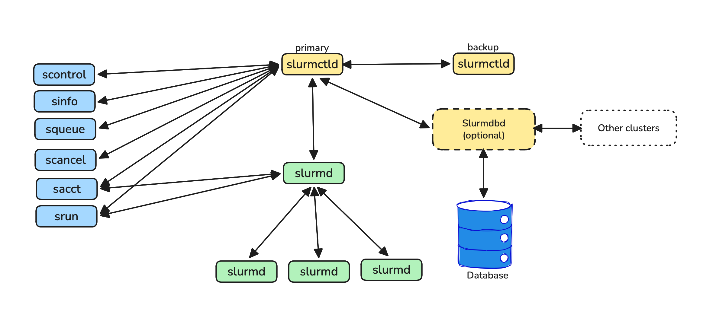
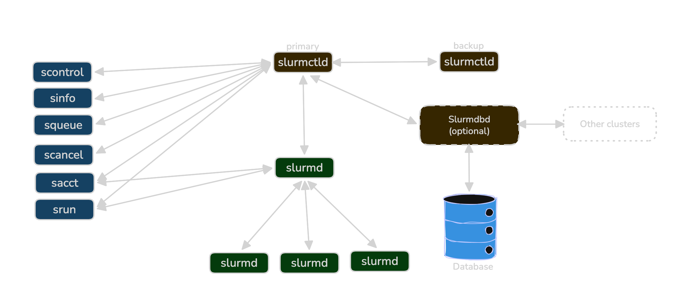
Figure 2.22: Slurm architecture overview: control daemon, node agents, and accounting daemon.

Slurm architecture overview: control daemon, node agents, and accounting daemon.

Architecture & daemons

Slurm is a centralized scheduler with per-node agents:

slurmctld - control daemon that computes priorities, places jobs, manages state; typically has a hot-standby backup.
slurmd - node-local agent that launches job steps, enforces cgroups and device binding, reports health.
slurmdbd - accounting daemon (optional but common) that persists jobs/associations/QoS to a DB for reporting and fairshare.

Scheduling & priority

Slurm uses a multifactor priority plugin plus backfill:

Priority is a weighted sum of components such as Age (queue wait), Fairshare (recent usage vs. target), QOS bonus, Partition bonus, and JobSize. Inspect with sprio -j <jobid>.
Backfill scans near-term idle windows and starts smaller/shorter jobs that won’t delay higher-priority reservations. Accurate --time and flexible constraints make you backfill‑friendly.

Partitions, QoS, accounts & associations

Partition: a queue backed by a set of nodes and limits (time, size, features). Jobs target one or more via -p p1,p2.
QoS: policy bundle-priority offsets, concurrency caps, preemption rules, max resources/time. See sacctmgr show qos (site-specific).
Accounts/Associations: project accounting and fairshare lineage tying users→accounts→QoS/limits. Check with sacctmgr show assoc where user=$USER.

Resources & features

GRES (generic resources) expose GPUs and other resources: --gres=gpu:1 or modern --gpus-per-task=1.
Features/constraints label nodes (e.g., a100, nvlink, ib). Use disjunctive constraints to widen placement: --constraint='a100|h100&nvlink'.
Licenses (optional plugin) model scarce tokens (e.g., EDA licenses) via --licenses=; similar to features but centrally counted.

The job model

sbatch script.sbatch submits a batch job. The script itself typically calls srun to launch ranks.
salloc creates an interactive allocation you can run srun steps inside.
srun without a prior allocation both allocates and launches a job step.
Jobs can be split into steps (e.g., one srun per phase) and arrays (--array=0-999%20) for sharded work. Chain with --dependency=afterok:<jid>.

Common states & preemption

Job states include:

PENDING (PD): The job has entered the queue but requested resources are not yet available (e.g., no free nodes, limits reached).
RUNNING (R): The job is currently executing with requested resources.
COMPLETED (CD): The job finished successfully according to the script.
COMPLETING (CG): The job is in the process of finishing.
FAILED (F): The job ended with a non-zero exit code.
CANCELLED (CA): The job was cancelled by the user or an administrator.
TIMEOUT (TO): The job reached its walltime limit.
PREEMPTED (PR): The job was stopped to make room for a higher-priority job.
NODE_FAIL (NF): The job terminated due to node failure; typically requeued automatically.
SUSPENDED (S): The job’s execution was paused and resources released.

Preemption is QoS‑driven; make jobs checkpoint‑aware and add --requeue so they restart cleanly after a USR1/TERM.

Common PENDING reasons

(Resources): Waiting for requested resources to become available.
(Dependency): Waiting for another job to complete/satisfy a condition.
(DependencyNeverSatisfied): Waiting for a dependency that can no longer be met; job must be cancelled.
(AssocGrpCpuLimit): Account or user has reached their allocated CPU quota.
(AssocGrpJobsLimit): Account or user has reached the concurrent job limit.
(ReqNodeNotAvail): A requested node is offline, reserved, or busy.

Cgroups & prolog/epilog

Sites often enable cgroup enforcement for CPUs/memory/GPUs and admin prolog/epilog scripts to prepare or clean nodes. If your process exceeds memory, the kernel/cgroup will OOM-kill it — size --mem honestly and monitor with sstat.

Operational cheat-sheet

The most common commands for managing jobs and inspecting cluster state. Many accept -o/--format strings for a more condensed view than the defaults.

sbatch <script>: Submit a script for asynchronous execution. Typically contains resource requests and srun steps.
squeue: View the queue (default: shows JobID, Partition, Name, User, State, Time, Nodes, Nodelist/Reason).
- Optimized view: squeue -o "%9i %9P %8j %8u %2t %12R %8M %C %b"
- Estimated start: squeue --start -j <jobid>
- Auto-refresh: squeue --iterate=N (refreshes every N seconds)
scancel <jobid>: Cancel one or more jobs (comma-separated) or send it a signal (e.g., scancel --signal=USR1 <jobid>).
scontrol show job <jobid>: View or modify Slurm state (nodes, partitions, jobs). scontrol suspend/resume <jobid> can pause/unpause execution.
sinfo: View status of partitions and nodes (e.g., idle, alloc, down, drain).
- Optimized view: sinfo -o "%P %a %l %D %G %f"
salloc: Request an interactive allocation; starts a shell on the allocated resource.
srun <app>: Launch job steps (usually within an sbatch or salloc environment). Handles resource requirements and task placement.
sacct: Query the accounting database for active or completed jobs.
- Optimized view: sacct -j <jobid> --format=JobID,State,Elapsed,MaxRSS,ExitCode
sstat: View real-time resource usage of a running job (CPU, RSS, VM).
sprio: View job priority breakdown (Age, Fairshare, QOS, etc.).
sview: Graphical user interface for cluster status, jobs, and partitions.
Node health: scontrol show node <nodename>

The sections that follow translate these mechanics into actionable guidance — how to request resources correctly, react to scheduler signals, and build pipelines that survive preemption and node failures.

2.4.2 Core Concepts

Schedulers enforce site policy while trying to keep expensive hardware busy. A little terminology goes a long way: understanding how queues are organized, how priority is calculated, and what “resources” really mean will make your jobs more placeable and your expectations more realistic. The same ideas exist in Kubernetes, but the knobs look different.

Partitions and QoS

Partitions logically group compute nodes and enforce resource limits (max time, node count, allowed users). QoS definitions layer on top: they govern priority offsets, resource ceilings, and preemption rules. Kubernetes achieves similar isolation through namespaces and resource quotas.

Practical guidance:

Target multiple partitions to widen placement: -p a100,h100 lets the scheduler choose whichever has capacity first.
Inspect limits before submitting: sinfo -o "%P %a %l %D %G" for partitions, sacctmgr show qos for QoS policies.
Reserve preemptible QoS for jobs that checkpoint quickly and handle USR1/TERM gracefully; use a non-preemptible QoS with an accurate --time for everything else.

A typical multi‑tenant Slurm site exposes several QoS classes with different trade‑offs:

QoS	Typical use	Trade‑offs
`debug`	Small, quick tests	Very short `--time`; high priority; low concurrency caps
`batch`	Normal training runs	Balanced priority; fairshare‑driven; moderate limits
`preempt`	Opportunistic large runs	Higher start chance; can be preempted; needs checkpoints

When in doubt, start with the “batch‑like” QoS for production runs and reserve debug/preempt for focused tests and opportunistic work that can tolerate interruption or stricter limits.

Priority and fairshare

Slurm favours users/projects that have consumed less recently and jobs that have waited longer. Accurate time limits and flexible constraints improve your position for backfill. Vanilla Kubernetes has no native backfill; similar effects come from realistic requests and flexible placement, or from a custom scheduler.

To improve your standing:

Inspect priority breakdown with sprio -j <jobid> — it shows age, fairshare, QoS, and partition contributions.
Keep --time honest — inflated walltimes don’t fit backfill gaps and delay your own start.
Use --nice to voluntarily lower priority for opportunistic or exploratory runs.
Avoid pinning to specific hostnames or rare features unless strictly required by the workload.

Resources are multi-dimensional

A job request has five independent dimensions — the scheduler must satisfy all of them simultaneously:

Dimension	Slurm flag(s)
Nodes / tasks	`--nodes`, `--ntasks-per-node`
CPU threads per rank	`--cpus-per-task`
Memory	`--mem-per-gpu` or `--mem`
GPUs per rank	`--gpus-per-task=1` or `--gres=gpu:N`
Node features / topology	`--constraint='a100\\|h100&nvlink'`

Key rules:

One rank per GPU is the standard for training: --ntasks-per-node=<gpus> --gpus-per-task=1.
Request features disjunctively (e.g., a100|h100) rather than exact hostnames — flexibility widens placement.
Avoid --exclusive unless the workload genuinely needs the full node; precise requests let the scheduler co-schedule other jobs and reduce your queue time.

Lifecycle

Jobs transition through states like PENDING (waiting), running, and exiting as COMPLETED, FAILED, CANCELLED, or TIMEOUT. On shared systems, preemption and node failures are normal events; design your jobs to be resilient to them.

squeue -j <jobid>                                              # live state during execution
sacct -j <jobid> --format=JobID,State,Elapsed,MaxRSS,ExitCode # post-completion triage

To enable automation to decide whether to requeue, resume, or fail fast: enable --signal and --requeue, trap signals for checkpointing, and ensure clear exit codes.

stateDiagram-v2
    direction LR
    [*] --> PENDING : sbatch / srun
    PENDING --> RUNNING : resources allocated
    PENDING --> CANCELLED : scancel
    RUNNING --> COMPLETED : exit 0
    RUNNING --> FAILED : non-zero exit
    RUNNING --> TIMEOUT : walltime exceeded
    RUNNING --> PREEMPTED : higher-priority job
    RUNNING --> NODE_FAIL : hardware fault
    PREEMPTED --> PENDING : --requeue
    NODE_FAIL --> PENDING : --requeue
    PREEMPTED --> FAILED : no requeue
    NODE_FAIL --> FAILED : no requeue
    COMPLETED --> [*]
    CANCELLED --> [*]
    FAILED --> [*]
    TIMEOUT --> [*]

2.4.3 Quickstart

If you’re new to Slurm, start with --nodes=1 --ntasks-per-node=1 --gpus-per-task=1 and a short walltime (30–60 minutes). Once that single-GPU job runs reliably, scale up and introduce arrays.

#!/usr/bin/env bash
#SBATCH -J train
#SBATCH -A <account>
#SBATCH -p <partition>
#SBATCH --qos=<qos>
#SBATCH --nodes=1
#SBATCH --ntasks-per-node=8
#SBATCH --gpus-per-task=1                # or: --gres=gpu:8 on sites without --gpus-per-task
#SBATCH --cpus-per-task=8
#SBATCH --mem-per-gpu=64G                # prefer explicit mem; avoid mem=0 if site disallows it
#SBATCH --time=06:00:00
#SBATCH --signal=B:USR1@120 --requeue
#SBATCH --output=logs/%x-%j.out

set -euo pipefail
trap 'echo "[${HOSTNAME}] USR1/TERM -> checkpoint"; python -m app.checkpoint --quick || true; scontrol requeue $SLURM_JOB_ID; exit 0' USR1 TERM
# Note: `app.checkpoint` is a placeholder. Replace with your actual checkpoint command/script.
trap 'echo "[${HOSTNAME}] EXIT cleanup"; rm -rf "${SLURM_TMPDIR:?}"/* || true' EXIT
sleep $((RANDOM%15))  # jitter to de-sync heavy I/O

export MASTER_ADDR=$(scontrol show hostnames "$SLURM_JOB_NODELIST" | head -n1)
export MASTER_PORT=${MASTER_PORT:-29500}

srun --gpu-bind=single:1 \
  python train.py \
    --master-addr "$MASTER_ADDR" \
    --master-port "$MASTER_PORT"
# Replace train.py with your entry point. For containerised runs see the Slurm Recipes section.

Use squeue --start -j <jobid> to preview the current backfill estimate.

2.4.4 Resource Requests: CPU, GPU, Memory, Time

Most scheduling friction comes from mismatched requests: asking for too much delays your start; asking for too little leads to throttling or failures. Treat resource requests as an engineering hypothesis-measure, adjust, and keep them honest. Where possible, make your job tolerant to a range of placements so the scheduler has more ways to run you.

CPUs per task

Properly allocate host threads to ensure dataloaders, tokenizers, and communication libraries remain busy without starving sibling ranks. Insufficient CPU allocation often manifests as sawtooth GPU utilization, indicating a bottleneck. Conversely, over-provisioning can negatively impact co-located jobs and even reduce your own throughput.

A good starting point is to set --cpus-per-task equal to the number of dataloader workers plus a few additional threads for orchestration. Remember to export OMP_NUM_THREADS=$SLURM_CPUS_PER_TASK and use srun --cpu-bind=cores to prevent CPU contention.

For workloads where simultaneous multithreading (SMT) is detrimental (e.g., tokenizers or certain ETL processes), consider adding #SBATCH --hint=nomultithread or #SBATCH --threads-per-core=1. Always validate the impact using tools like mpstat or iostat.

Memory headroom

Set memory per node or per GPU with enough headroom for model weights, caches, NCCL/UCX communication buffers, and dataloader workers. Too little memory surfaces as OOM kills or aggressive page-cache eviction; too much just increases your queue wait. Prefer explicit per-GPU requests (--mem-per-gpu) over --mem=0, which some sites disallow. Track actual consumption with sstat -j $SLURM_JOB_ID --format=MaxRSS,AveRSS and size your limit to peak usage plus a 10–20% buffer.

GPUs per rank and model

For optimal training performance, map one process (rank) to one GPU, unless your framework explicitly handles multiplexing. While full GPUs are preferred for large-scale training, consider using MIG or MPS for smaller fine-tuning tasks and inference. In Slurm, ensure a 1:1 binding between ranks and devices by setting --ntasks-per-node=<gpus> with --gpus-per-task=1, and include srun --gpu-bind=single:1. If --gpus-per-task is unavailable, use --gres=gpu:1 as an alternative.

Topology and constraints

To accelerate job placement, constrain your requests by GPU generation or node features (e.g., A100/H100, NVLink, IB). Always prefer disjunctive constraints, such as --constraint='a100|h100&nvlink&ib', over exact hostnames, reserving hostname-specific requests only for debugging. You can discover available features using sinfo -o "%N %f".

Time limit

Setting a realistic walltime is crucial. Accurate time limits in Slurm improve your job’s chances of backfilling and reduce idle cluster time. Conversely, overly long or padded limits can delay your job’s start and block others. Conduct a short pilot run to estimate throughput, then set --time accordingly. Optionally, use --time-min to enable earlier backfill starts when less time is available. Preview estimated start times with squeue --start -j <jobid>.

Advance notice

For graceful job termination and requeueing, request a pre-timeout signal in Slurm using --signal=B:USR1@120 (120 seconds before the job ends). Implement a signal trap to checkpoint your progress and then call scontrol requeue $SLURM_JOB_ID to restart cleanly. Additionally, an EXIT trap ensures proper cleanup of scratch directories and flushing of logs upon normal termination.

Interconnect

If your job relies on collective communication (e.g., DDP, ZeRO), verify that compute nodes are equipped with IB/RDMA and that your container or module stack exposes it. High all-reduce times relative to computation often indicate poor interconnect performance. To diagnose:

export NCCL_DEBUG=INFO               # log transport selection and ring topology
export NCCL_ASYNC_ERROR_HANDLING=1   # fail fast on transport errors
export NCCL_IB_HCA=mlx5_0            # pin to a specific HCA when multiple exist
export NCCL_SOCKET_IFNAME=ib0        # choose the correct NIC when multiple fabrics are present

Storage locality

Optimize data access by training from large, sequentially readable shards and staging frequently accessed data to node-local SSD or RAM-disk. Avoid inefficient random access to numerous small files on shared filesystems. Utilize $SLURM_TMPDIR for ephemeral scratch data and ensure it’s cleaned up upon job exit to maintain node hygiene.

Concurrency and blast radius

To protect the cluster and maintain predictable runtimes, cap your job array width and stagger the starts of individual tasks. For example, use --array=0-999%20 to limit concurrent tasks and add a small random sleep (sleep $((RANDOM%15))) at the beginning of your script to de-synchronize heavy I/O phases across tasks.

2.4.5 Planning Compute Budgets and GPU‑Hours

Schedulers and quotas exist because GPU time is scarce. Thinking in GPU‑hours (or node‑hours) helps you design experiments that fit both your project’s budget and the shared cluster. This section gives you simple rules to estimate cost, read your usage, and plan runs so you don’t burn the budget on a few unlucky experiments.

Understanding and Estimating GPU‑Hours

Many HPC sites track usage per account/project and enforce fairshare or hard quotas. Even without explicit billing, there is always an implicit budget: how much cluster time your team can reasonably consume. GPU‑hours are a convenient common unit for measuring this, defined as:

GPU‑hours = (number of GPUs) × (walltime in hours)

For multi‑node jobs, multiply by the total GPUs across all nodes (e.g., 4 nodes × 8 GPUs/node × 6 h = 192 GPU‑hours). Thinking in GPU‑hours helps you:

Compare the cost of different job sizes (e.g., 8 GPUs for 4 h vs. 16 GPUs for 2 h).
Plan how many experiments fit into a fixed project budget.
Justify trade‑offs between model size, resolution, batch size, and search breadth (number of runs).

Before launching a large run, conduct a short pilot to measure real walltime and then estimate the cost:

gpu_hours ≈ (nodes × gpus_per_node × elapsed_hours)

For example:

1 node × 4 GPUs × 3 h → 12 GPU‑hours
4 nodes × 8 GPUs × 6 h → 192 GPU‑hours
8 nodes × 8 GPUs × 24 h → 1,536 GPU‑hours

After a job completes, you can inspect the actual elapsed time and allocated GPUs using Slurm’s sacct command:

sacct -j <jobid> --format=JobID,Elapsed,AllocTRES%40,State

AllocTRES will include GPU counts (e.g., gres/gpu=32). Multiply by the elapsed hours to calculate the realized GPU‑hours for that job.

From experiment grids to budget

Hyperparameter sweeps and ablation studies are notorious budget sinks. Rather than launching a massive grid blindly, work backward from a target budget:

Estimate unit cost: Calculate the GPU‑hours for a single run.
Set a cap: Determine the total GPU‑hours affordable for the experiment family (e.g., 2,000 GPU‑hours).
Calculate capacity: Compute max_runs ≈ floor(budget / cost_per_run).
Design the grid: Select the most critical hyperparameters to fit within max_runs.

Once you have a cap, apply these patterns to maximize value:

Cheap proxies: Use smaller models, fewer steps, or lower resolutions to prune bad candidates early.
Coarse‑to‑fine search: Cast a wide, shallow net first, then drill down with expensive runs only on promising candidates.
Reuse artifacts: Share checkpoints and preprocessed data across runs to avoid redundant computation.
Statistical significance: Prioritize multiple seeds on smaller jobs over single, gigantic runs, especially during debugging.

Reading project usage

While you typically cannot change quotas as a standard user, you can—and should—monitor your consumption to adjust behavior.

To audit specific jobs or project-wide usage:

# Per-job view
sacct -j <jobid> --format=JobID,Elapsed,AllocTRES%40,State -P

# Per-account summary (if allowed)
sacct -A <account> --format=JobID,Elapsed,AllocTRES%40,State -P > account_usage.csv

Importing this data into a spreadsheet or Python script allows you to aggregate GPU‑hours by week or month, quickly revealing which experiments are dominating the budget. Additionally, check if your site offers sreport or web portals to track your standing against fairshare policies.

Designing experiments under a fixed budget

When resources are finite, efficiency is a design constraint. Adopting these heuristics can stretch a fixed budget significantly:

Pilot before scaling: Always run small‑scale pilots to verify throughput and convergence speed before committing to full‑scale training.
Right‑size resources: Avoid debugging on 64 GPUs. Start with 1–4 GPUs and scale out only after code and I/O stability are confirmed.
Default to modest limits: Configure launch scripts to default to low node counts, requiring deliberate overrides for large‑scale runs.
Cap walltimes: Shorter jobs with reliable checkpointing improve scheduler backfill opportunities and minimize the cost of mid‑run failures.
Prioritize by ROI: Rank experiments by their expected value versus cost. Run high‑impact, low‑cost ideas first.
Standardize baselines: Agree on a shared set of baseline configurations to prevent team members from wasting cycles reinventing the wheel.

Budget‑aware guardrails to bake into tooling

The most effective way to enforce these practices is to encode them into your submission scripts and internal tooling:

Threshold warnings: Alert users when a job request exceeds a specific cost (e.g., > 512 GPU‑hours).
Grid limits: Block the launch of hyperparameter grids that exceed a daily budget unless an explicit --force flag is used.
Cost logging: Record estimated GPU‑hours in experiment metadata, enabling post‑mortems to evaluate cost versus benefit.
Structural preferences: Design tools to favor “many small” jobs (e.g., smaller arrays, shorter walltimes with restarts) over risky, monolithic allocations.

Treating GPU‑hours as a first‑class resource—just like memory or disk space—makes your usage of shared infrastructure more efficient and easier to justify to stakeholders.

2.4.6 Lifecycle Signals: How to Respond

Schedulers and kernels communicate through states and signals. Learning to interpret these signals allows you to react quickly, wasting less GPU time and building naturally resilient jobs. Treat this section as a troubleshooting playbook to automate within your launchers and signal traps.

PENDING: Resource Starvation

If a job lingers in PENDING, inspect the specific blocker:

squeue -j <jobid> -o '%T %R'    # show state and reason

To unblock it, try adjusting the “smallest lever” first: loosen constraints (e.g., allow multiple GPU generations), shorten the requested time limit, or split a monolithic job into phases. If the reason is policy-based (Quota/QoS), you may need to coordinate with platform owners.

RUNNING: Performance Degradation

If a job is RUNNING but throughput is low, check your resource binding. Ensure one rank per GPU, stable CUDA_VISIBLE_DEVICES, and correct NUMA locality. If GPU utilization is low while CPUs are pegged, the bottleneck is likely data loading; increase dataloader threads or improve I/O locality.

nvidia-smi dmon -s u              # watch GPU utilization live
srun --cpu-bind=cores --gpu-bind=single:1 ...   # correct launch flags

FAILED or TIMEOUT

Jobs should fail loudly and cleanly. Ensure your script exits with meaningful error codes and messages. For timeouts, the goal is a clean save-and-exit rather than a hard kill; ensure your signal traps perform a quick checkpoint before the walltime expires. Always write checkpoints atomically (write to temp, then rename) so that reruns are idempotent. Triage post-mortem using sacct -j <jobid> --format=JobID,State,ExitCode.

PREEMPTED or NODE_FAIL

Treat preemption not as an error, but as a routine pause. Handle signals by checkpointing promptly and requeuing automatically. If specific nodes are “flapping” (repeatedly failing), use --exclude to temporarily blacklist them and alert admins. Combine the --requeue flag with a SIGUSR1 trap to handle these interruptions gracefully.

Out-of-Memory Kills

Distinguish immediately between Host OOM and Device OOM.

Device (GPU) OOM: Usually caused by model or batch sizing. Reduce batch size, sequence length, or use activation checkpointing.
Host (CPU) OOM: Manifests as kernel kills. This often comes from aggressive dataloading. Raise the --mem request or reduce the number of dataloader workers.

2.4.7 Queue & Backfill Optimization

Queue time isn’t random; it’s about fit. The scheduler can start your job quickly when your request is truthful (accurately sized), flexible (allowing more placement options), and backfill-friendly (with an accurate time estimate). Leveraging these factors can significantly reduce your wait time without needing to game the system.

How backfill works

Backfill looks for near‑term idle gaps and starts jobs that fit the gap without delaying higher‑priority reservations. Two practical rules follow:

Keep --time honest; padded limits do not fit in gaps.
Make placement flexible (multiple partitions, disjunctive constraints) so more gaps become usable.

gantt
    title Backfill fills idle gaps before the high-priority job can start
    dateFormat HH:mm
    axisFormat %Hh

    section Nodes 1-4
    J_long (running)        :active, 00:00, 06:00

    section Nodes 5-8
    J_medium (running)      :active, 00:00, 03:00
    J_small_A (backfilled)  :done,   03:00, 05:00
    J_small_B (backfilled)  :done,   03:00, 06:00

    section All 8 nodes
    J_priority (PENDING to RUNNING) :crit, 06:00, 10:00

You can always check the current estimate with:

squeue --start -j <jobid>            # predicted start time if limits/shape stay the same
sprio -j <jobid>                      # priority breakdown (age, fairshare, qos, etc.)

Keep time limits accurate

Do a short pilot and measure real throughput, then compute walltime with a small margin:

walltime ≈ (total_steps × seconds_per_step) / 3600  + 10–20% margin

Example. If 1,000 steps at 2.7 s/step: (1000×2.7)/3600 ≈ 0.75 h. Request --time=00:50:00 to be backfill‑friendly, not --time=03:00:00.

Use `--time-min` to accept shorter windows

You can specify a preferred time and a minimum acceptable time:

sbatch \
  --time=04:00:00 \
  --time-min=02:00:00 \
  train.sbatch

This lets the scheduler start you earlier if only a 2‑hour slot is free. Your job must handle graceful stop/checkpoint.

Widen placement with constraints and partitions

Let the scheduler place you on more nodes by expressing alternatives:

-p a100,h100 \
--constraint='a100|h100&nvlink'      # either A100 or H100, but must have NVLink

Tips:

Prefer features over hostnames; host pinning narrows placement and increases wait.
Keep quoting correct for complex expressions (use single quotes to avoid shell expansion).

Make your job shape easy to place

Schedulers place shapes: nodes, GPUs/node, CPUs/task, memory. Shapes that fit easily start sooner.

One rank per GPU: --ntasks-per-node=<gpus> --gpus-per-task=1 and srun --gpu-bind=single:1.
Avoid --exclusive unless you truly need full nodes; precise requests co‑schedule better.
Match CPU & memory to your use: don’t request odd combos that leave unusable fragments (e.g., all RAM with 1 GPU on an 8‑GPU node).
If your site lacks --gpus-per-task, use --gres=gpu:1 (same intent).

Choose preemptible QoS only when ready

Preemptible queues can start faster if you can stop/resume cleanly. Must‑haves:

Checkpoint quickly on USR1/TERM (--signal=B:USR1@120 --requeue and a tested trap).
Checkpoints are small/atomic (write to temp then rename).
Array width is capped so retries don’t stampede the filesystem. Nice‑to‑haves: staggered start jitter, per‑rank logs with last successful step.

Plan reservations for very large runs

For many nodes/GPUs, rehearse on 1–2 nodes first (container, I/O, ports, NCCL). When ready, coordinate an advance reservation and submit with:

#SBATCH --reservation=<name>

Document the image digest, git SHA, and shard manifest so the rehearsal matches production.

Separate ETL/evaluation from training

ETL and evaluation rarely need expensive GPUs. Run them as smaller, capped arrays and keep the largest slots for training.

#SBATCH --array=0-999%20     # cap concurrency to protect the scheduler & filesystem
sleep $((RANDOM%15))         # jitter to de‑sync metadata bursts

Move heavy parsing or tokenization to CPU partitions when possible; stage data to $SLURM_TMPDIR for locality.

Diagnosing a long PENDING job

Inspect reason & shape:

squeue -j <jobid> -o '%i %t %R %D %C %m %b'
scontrol show job <jobid> | sed -n '1,60p'

Improve fit in this order (smallest change first):
- Tighten --time (or add --time-min).
- Widen constraints: drop rare features; allow multiple GPU gens or partitions.
- Reduce nodes (scale up ranks per node) if feasible.
- Right‑size memory (prefer --mem-per-gpu over --mem=0 where disallowed).
Re‑submit with the improved shape; keep a comment for traceability:

sbatch --comment "fit-tuned v2" train.sbatch

Respect scheduler scalability and submission rates

Central schedulers like slurmctld have finite capacity. Overloading them increases everyone’s time-to-start, including yours.

Use job arrays instead of individual jobs — --array=0-999%20 submits one scheduler entry instead of 1,000, reducing overhead.
Pace submissions and requeues — avoid tight while loops that call squeue or sbatch repeatedly within seconds.
Respect site limits — check MaxArraySize and project/job concurrency caps; ask admins if unsure.
Reuse allocations for multi-step work — run several sequential steps inside a single job rather than submitting a new job per step.

Healthy scheduler load makes everyone’s time‑to‑start more predictable, including yours.

Anti-patterns that increase wait time

Anti-pattern	Why it hurts
Inflating `--time` “just in case”	Padded limits don’t fit backfill gaps; delays your own start
Pinning to specific hostnames	Narrows placement to a handful of nodes; almost always unnecessary
`--exclusive` for single-GPU jobs	Wastes co-scheduling opportunity on multi-GPU nodes
Requesting all node memory	Leaves unusable fragments; blocks co-scheduled jobs
Wide arrays with no cap or jitter	Metadata storms slow the filesystem for everyone, including you

2.4.8 Placement & Topology Optimizations

Many “mysterious slowdowns” trace back to where ranks land and which GPUs/CPUs they talk to — collective communication and host–device transfers are extremely sensitive to placement: a great model with poor binding often underperforms a smaller model with correct binding.

Deterministic binding

Two ranks attached to the same GPU (or to different GPUs than expected) cause oversubscription, memory pressure, and sometimes deadlocks in collectives. Make the rank → GPU → CPU mapping explicit and verify it early.

Ask Slurm to bind one GPU per task and pin CPU cores for each task:

srun --ntasks-per-node=<gpus> --gpus-per-task=1 \
     --gpu-bind=single:1 --cpu-bind=cores ...
# If your site lacks --gpus-per-task, use: --gres=gpu:1

Log the resolved mapping at startup so you can prove where each rank landed:
```
echo "HOST=$(hostname) RANK=$RANK LOCAL_RANK=$LOCAL_RANK WORLD_SIZE=$WORLD_SIZE CUDA_VISIBLE_DEVICES=$CUDA_VISIBLE_DEVICES"
```
For PyTorch, also print the device name once per rank.

Common pitfalls to avoid: mixing mpirun with srun (double‑launch breaks binding), and changing CUDA_VISIBLE_DEVICES inside your script after Slurm has set it.

NUMA and sockets

CPUs and memory are split across sockets (NUMA). When a rank’s threads or memory allocations cross to the other socket, you pay extra latency and lose bandwidth — 10–30% regressions are common. Keep each rank’s CPU threads and memory on the socket that feeds its GPU.

Use local pinning and sized threads:

srun --cpu-bind=cores --mem-bind=local ...
export OMP_NUM_THREADS=$SLURM_CPUS_PER_TASK
numactl --hardware     # inspect NUMA nodes and distances when debugging

If dataloaders spill across sockets, either reduce worker count or raise --cpus-per-task to keep locality.

NVLink / NVSwitch grouping

Not all intra‑node links are equal. NVLink/NVSwitch provide far more bandwidth than PCIe, so tensor/pipeline parallel groups should live on GPUs that are tightly connected. On 8‑GPU nodes without NVSwitch, treat them as two 4‑GPU islands (e.g., 0–3 and 4–7) for TP/PP groups; reserve inter‑node links for data parallel. On NVSwitch systems (A100/H100 DGX‑class), connectivity is uniform, though CPU locality still matters.

Inspect the link matrix:

nvidia-smi topo -m

Inter-node readiness with RDMA and InfiniBand

Multi‑node training depends on fast collectives — if RDMA/IB isn’t used, traffic falls back to TCP and step time balloons. Confirm the intended fabric and give NCCL minimal hints when multiple NICs are present:

export NCCL_ASYNC_ERROR_HANDLING=1   # fail fast on transport errors
export NCCL_SOCKET_IFNAME=ib0        # pick the correct interface name on your site
export NCCL_IB_HCA=mlx5_0            # select HCA when multiple exist
export MASTER_ADDR=$(scontrol show hostnames "$SLURM_JOB_NODELIST" | head -n1)
export MASTER_PORT=${MASTER_PORT:-29500}

A tiny warm‑up collective flushes obvious issues before real work:

python - <<'PY'
import os, torch, torch.distributed as dist
if torch.cuda.is_available():
    dist.init_process_group('nccl', rank=int(os.environ['RANK']), world_size=int(os.environ['WORLD_SIZE']))
    x = torch.ones(1, device='cuda') * (int(os.environ['RANK'])+1)
    dist.all_reduce(x)
    print('all_reduce_ok', x.item())
PY

If you see hangs, try a different MASTER_PORT and verify firewalls aren’t blocking the rendezvous.

MIG / MPS guidance

MIG slices reduce the memory/SMs available to a process and MPS adds sharing overhead. They’re great for small fine‑tunes or high‑concurrency inference, but they can starve large models.

When it fits, request MIG via site‑specific GRES labels, for example:

#SBATCH --gres=gpu:1g.10gb:1   # example; confirm exact label names on your site

If MIG isn’t exposed to Slurm, you can’t rely on --gpus-per-task to pick a slice-coordinate with admins to avoid collisions.

Topology inspection quick refs

nvidia-smi topo -m      # GPU↔GPU/CPU connectivity and link type
numactl --hardware      # NUMA nodes and distances
hwloc-ls --of console   # CPU/GPU/PCIe topology (if available)

Advanced: NCCL/UCX tuning

Defaults are usually sufficient; mixed fabrics (multiple HCAs, RoCE vs IB, containers) sometimes need extra hints. Change one variable at a time and record the effect (examples/sec, all‑reduce time).

Common, generally safe hints:

export NCCL_ASYNC_ERROR_HANDLING=1        # detect errors instead of hanging
export NCCL_SOCKET_IFNAME=ib0             # choose the right NIC when multiple exist
export NCCL_IB_HCA=mlx5_0                 # pin to a specific HCA
export NCCL_NET_GDR_LEVEL=PHB             # constrain GPUDirect RDMA level on tricky platforms
export UCX_TLS=rc,sm,self                 # prefer reliable connection + shared memory
export UCX_NET_DEVICES=mlx5_0:1           # choose device/port (dual‑rail clusters)

Over‑constraining can reduce performance, so revert to defaults if a tweak makes things worse.

Troubleshooting cheat‑sheet

Symptom	Likely cause	Next step
Two ranks pick the same GPU or crash at startup	No deterministic binding; double‑launch	Use `srun --gpu-bind=single:1`; avoid mixing `mpirun` and `srun`; log mapping
GPUs idle while CPUs sit at 100%	NUMA mismatch or too few CPU threads	Add `--cpu-bind=cores --mem-bind=local`; right‑size `--cpus-per-task`
Multi‑node steps much slower than single‑node	RDMA not used / wrong NIC selected	Set `NCCL_SOCKET_IFNAME` / `NCCL_IB_HCA`; run micro all‑reduce; check firewall/ports
Good intra‑node, poor TP/PP scaling	TP/PP spans weak PCIe links	Group within NVLink islands (e.g., 0–3 / 4–7)
Unpredictable latency under concurrency	MPS/MIG oversubscription	Reduce sharing or move heavy jobs to full GPUs

2.4.9 Containers on HPC

On HPC, containers give you reproducible user‑space while staying compatible with host drivers. The catch is that many compute nodes don’t have internet access (and even when they do, registries can be rate‑limited). This changes how you build, distribute, verify, and launch images. Below are robust patterns for both scenarios and the safeguards that keep runs predictable.

Choose Singularity / Apptainer for scheduler‑friendly execution

Note

Singularity is now known as Apptainer under the Linux Foundation. Most commands are compatible or aliased (e.g., singularity often invokes apptainer), but we refer to “Singularity” here as it remains the common vernacular on many legacy HPC systems.

Singularity/Apptainer runs containers as your own UID, integrates with Slurm cgroups, and packages images as immutable SIF files. That immutability is a feature: you can pin an exact artifact, verify it, and get bit‑for‑bit identical runs. GPU pass‑through is handled with --nv, and accounting/cgroups work cleanly.

Compute nodes with internet access

Less common, but when allowed you can pull/convert on the fly-still prefer pinned, verified artifacts so tags can’t drift.

Pin by digest:

singularity pull \
  docker://nvcr.io/nvidia/pytorch:24.08-py3@sha256:<digest>
# → pytorch_24.08-py3_<digest>.sif

Keep a fast cache to avoid hammering registries during arrays:

export SINGULARITY_CACHEDIR=/scratch/$USER/singularity-cache

Keep registry credentials out of job scripts if using private repos. Authenticate on a login/builder node, then convert to SIF once and reuse the SIF in jobs.

Even with internet access, the safer pattern is to pull once on a login/builder node, produce a SIF, and reuse that single artifact across jobs.

Compute nodes without internet access

Here the container must be present before the job starts consuming the network.

Build or pull on a connected machine (CI, workstation, or login node) and convert to SIF:

singularity pull myenv_pytorch_24.08.sif \
  docker://nvcr.io/nvidia/pytorch:24.08-py3@sha256:<digest>

Stage SIFs to a shared, read‑only location (e.g., /shared/containers/) or copy to node‑local scratch at runtime:
```
IMAGE=/shared/containers/myenv_pytorch_24.08_<digest>.sif
STAGED=$SLURM_TMPDIR/$(basename "$IMAGE")
[[ -f "$STAGED" ]] || cp "$IMAGE" "$STAGED"
```
For very large images at scale, coordinate with admins to fan‑out the SIF (e.g., site prolog or sbcast).
Verify provenance before execution (SIF signatures/keys), especially for CI‑produced images:
```
singularity verify $IMAGE   # requires trusted public keys
```

Image distribution patterns that scale

Shared read‑only path: versioned, content‑addressed names like /shared/containers/<name>@sha256_<digest>.sif.
Node‑local cache: copy once into $SLURM_TMPDIR per node to cut network hot spots.
Cluster broadcast (admin‑assisted): use site tools (e.g., sbcast) or prolog scripts for large deployments.

Execution safeguard checklist

Pin the image by digest and verify signatures; SIFs are immutable-use that to your advantage.
Driver/library match: --nv pulls host CUDA/NCCL/driver into the container; keep container user‑space compatible with host versions.
Stable environment: prefer --cleanenv --contain so stray host modules/vars don’t leak. Set runtime vars via SINGULARITYENV_… (e.g., SINGULARITYENV_NCCL_DEBUG=WARN).
Bind intentionally: read‑only datasets and isolated scratch keep runs reproducible:
```
--bind /datasets:/datasets:ro --bind "$SLURM_TMPDIR:/scratch"
```
Respect cgroups: Slurm enforces CPU/mem/GPU; honest requests avoid OOM kills.
Pre‑flight once: do a tiny model load or collective on one node to catch ABI/driver mismatches before scaling.

Launching with Slurm and Singularity

srun --nodes=2 --ntasks-per-node=8 --gpus-per-task=1 \
  singularity exec --nv --cleanenv --contain \
  --bind /datasets:/datasets:ro --bind "$SLURM_TMPDIR:/scratch" \
  /shared/containers/myenv_pytorch_24.08_<digest>.sif \
  torchrun --nproc_per_node=$SLURM_NTASKS_PER_NODE \
           --nnodes=$SLURM_NNODES \
           --rdzv_backend=c10d \
           --rdzv_endpoint=$MASTER_ADDR:$MASTER_PORT \
           train.py

If you staged the image to node‑local scratch, swap the SIF path with $SLURM_TMPDIR/myenv.sif.

Container alternatives integrated with Slurm

Some sites install container integrations that run OCI images directly:

Pyxis (NVIDIA) + Enroot - avoids SIF conversion and works with GPUs:
```
srun \
  --container-image=nvcr.io/nvidia/pytorch:24.08-py3@sha256:<digest> \
  --container-mounts=/datasets:/datasets:ro,$SLURM_TMPDIR:/scratch \
  --container-remap-root \
  python train.py
```
On clusters without internet access, pre‑import the image to an Enroot rootfs (.sqsh) on a shared path and reference it via: --container-image=/shared/containers/pytorch_24.08.sqsh.
Other options you may encounter: Shifter and Charliecloud. Flags and offline staging are site‑specific, but the same “pin, stage, verify” principles apply.

2.4.10 Filesystems & I/O Hygiene

Your I/O pattern can make or break GPU utilization. Shared filesystems excel at large, sequential reads and writes; they struggle with storms of tiny, random operations. When metadata servers are saturated or readers seek all over the disk, GPUs stall waiting for input. Organize data and access so storage becomes a quiet partner rather than the bottleneck.

Prefer large, sequential shards

Small files create a heavy metadata tax (open/close, stat/readdir); large shards amortize that cost and let storage stream at full bandwidth. Use WebDataset tar shards, Parquet, or RecordIO instead of millions of tiny files, and read them sequentially.

Sizing targets

Shard size: 128 MB–1 GB per shard (training) and 64–256 MB for inference/validation where latency matters.
Parquet row groups: 64–256 MB so each read pulls contiguous data and vectorized scans stay efficient.
Compression: choose zstd or lz4 for a good CPU/I/O trade‑off; avoid deep gzip when CPUs are busy.

Layout and ordering

Keep homogeneous content together (e.g., similar sequence lengths) to reduce padding and seeking.
Prefer few big shards over many tiny ones; if you must split by class or language, aim for tens or hundreds of shards, not thousands.
For WebDataset, generate tar shards once and reuse them; randomize by shard order first, then by sample order within each shard.

Measure with iostat -xm 1, nvidia-smi dmon -s pucm, and per‑step dataloader timings; if GPUs wait while disks are idle, you’re not reading sequentially or the shards are too small.

Stage hot data locally

Staging to node‑local storage (NVMe or $SLURM_TMPDIR) avoids reading the same bytes repeatedly over the network and decouples job throughput from shared FS peaks. Stage once per node, read many times.

# Example: stage once, then atomically swap into place
set -euo pipefail
SRC=/shared/datasets/fineweb2/train_shards
DST=$SLURM_TMPDIR/fineweb2
TMP=${DST}.tmp

if [[ ! -d "$DST" ]]; then
  mkdir -p "$TMP"
  rsync -av --partial --inplace --info=progress2 "$SRC/" "$TMP/"
  mv -T "$TMP" "$DST"   # atomic rename
fi

# Use local path in the job
export DATA_ROOT="$DST"

Safeguards: leave enough free space on $SLURM_TMPDIR, clean it on EXIT, and prefer read‑only mounts for inputs to avoid accidental writes.

Throttle readers and stagger starts

Readers can easily overwhelm metadata servers; cap worker count and add jitter to smooth bursts across the cluster.

PyTorch DataLoader: start with num_workers=2–4 per rank, prefetch_factor=2, persistent_workers=True; raise gradually while observing FS load.
WebDataset: cap resampled pipelines; use workers judiciously and enable cache_dir only on local disks.
Stagger large arrays: limit width (--array=0-999%20) and add a small random sleep at start: sleep $((RANDOM%15)) to de‑sync metadata bursts.
Limit prefetch depth: long prefetch queues hide problems and amplify stampedes when shards rotate.

Monitoring tip: watch iostat, FS‐specific tools (e.g., lfs df -h on Lustre), and application logs for queueing at “open/read” stages.

Write checkpoints atomically

Half‑written checkpoints waste time and may corrupt progress. Writing atomically ensures that any consumer sees either the old checkpoint or the new one — never an in‑between file.

Write to a temporary path on the same filesystem, fsync, then atomic rename into place (Python os.replace).
Keep a tiny manifest (JSON) that records the last complete step/epoch and the file name; this makes resumption unambiguous.
Prefer fewer, incremental checkpoints over frequent full snapshots to reduce I/O volume.

Python sketch

import json, os, tempfile

def atomic_write(path: str, data: bytes):
    d = os.path.dirname(path)
    fd, tmp = tempfile.mkstemp(dir=d, prefix='.partial_', suffix='.tmp')
    try:
        with os.fdopen(fd, 'wb') as f:
            f.write(data)
            f.flush()
            os.fsync(f.fileno())
        os.replace(tmp, path)  # atomic on same filesystem
    finally:
        if os.path.exists(tmp):
            os.unlink(tmp)

# Update manifest
with open('checkpoint_manifest.json', 'w') as f:
    json.dump({'last_step': step, 'file': ckpt_path}, f)

Align shard counts with consumers

To optimize data throughput and minimize both straggler processes and cache thrashing, it’s crucial to align the number of data shards with your consumers. The goal is to ensure each consumer can process whole shards with minimal overlap and efficient resource utilization.

A “consumer” in this context is defined by the product of your Slurm array width, the number of nodes, and the ranks per node (i.e., array width × nodes × ranks per node).

Ideally, you should aim for a number of shards that is approximately k × consumers, where k is a small integer like 2-4. This allows each processing rank to cycle through several distinct shards without contention, promoting better data locality and reducing I/O bottlenecks.

Whenever possible, strive for even divisibility between shards and consumers. If perfect divisibility isn’t achievable, implement a work-stealing or deterministic round-robin assignment strategy to distribute the workload evenly and prevent hot spots.

To facilitate deterministic assignment of shards, maintain a manifest (e.g., a text file or CSV) that lists and indexes your shards by an integer. This allows Slurm array tasks to reliably map SLURM_ARRAY_TASK_ID to a specific subset of shards.

Example mapping

# N shards, M consumers; each task gets every M‑th shard starting at its index
TASK_ID=${SLURM_ARRAY_TASK_ID:-0}
python - <<'PY'
import os, glob
M = int(os.environ.get('WORLD_SIZE', os.environ.get('SLURM_ARRAY_TASK_MAX', '1')))+1
T = int(os.environ.get('SLURM_ARRAY_TASK_ID', '0'))
shards = sorted(glob.glob(os.environ['DATA_ROOT']+'/shard-*.tar'))
assigned = shards[T::M]
print('\n'.join(assigned))
PY

Advanced: Filesystem specifics

Lustre (MDT/OST striping). Stripe settings are crucial in Lustre as they dictate how files are distributed across Object Storage Targets (OSTs). For optimal performance with large sequential files, employ a moderate stripe count and a larger stripe size to maintain high throughput without overburdening metadata servers. You can inspect current stripe settings with lfs getstripe <file_or_dir> and check capacity using lfs df -h. When dealing with big tar or Parquet files, consider setting stripes like lfs setstripe -S 8M -c 4 <dir> (note: this is an example and should be site-specific); avoid -c -1 unless explicitly advised, as it can cause contention across all OSTs. Additionally, keep shard directories shallow to prevent metadata server (MDT) overload from excessively large directory listings.

GPFS / IBM Spectrum Scale. In GPFS (IBM Spectrum Scale), the directory layout significantly impacts performance because its metadata system scales more efficiently with a greater number of smaller directories rather than one monolithic directory. Therefore, prefer deeper directory trees, such as /data/lang=it/part=0000/, over flat structures. Focus on using larger files accessed sequentially, and minimize the count of small files to reduce metadata lock contention. GPFS often employs dynamic readahead, so sequential access patterns naturally assist the system in optimizing data delivery.

General diagnostics. When server-side settings are beyond your control, concentrate on optimizing client-side behavior. This includes ensuring large, sequential reads, limiting concurrency where possible, using shallow directory traversals, and staging frequently accessed “hot” data sets to local scratch storage for faster access.

2.4.11 Observability & Post‑mortems

What is not measured cannot be debugged or improved. Lightweight, consistent logging and metrics turn one‑off successes into repeatable pipelines and failures into fast fixes. HPC jobs are often short‑lived and distributed; you need just enough signal to reconstruct what happened without adding overhead or flooding shared filesystems.

Standardize run directories

Adopt a predictable layout and include the Slurm JobID (and Array Task ID) in paths so you can grep/compare across runs. A stable layout also makes post‑run collation trivial.

Example layout

<project_root>/runs/
  └── <run_name>__job=<JOBID>__task=<TASKID>/
      ├── config/
      │   ├── config.yaml              # full training/runtime config
      │   └── slurm_env.json           # selected Slurm env vars
      ├── logs/
      │   ├── rank-000.out             # structured stdout/stderr per rank
      │   ├── rank-000.metrics.jsonl   # 1 line = 1 metric sample (JSON)
      │   └── slurm-%x-%j.out          # scheduler logs
      ├── metrics/
      │   └── summary.csv              # post-run rollups (per minute)
      ├── checkpoints/
      │   └── ckpt_step_012345.safetensors
      ├── provenance/
      │   ├── git.txt                  # commit, dirty state
      │   ├── image.txt                # SIF path or container digest
      │   └── pkg-manifest.txt         # pip/conda list (optional)
      └── exit_info.json               # exit_code, reason, last_checkpoint

Create this tree at startup; never rely on default working directories that may vary across steps/nodes.

Emit per‑rank context

Record enough context so a single log line tells you who wrote it and where it ran — distributed jobs fail asymmetrically (one rank hangs, another OOMs).

Bash at startup

export RUN_DIR="$PROJECT_ROOT/runs/${RUN_NAME}__job=${SLURM_JOB_ID}__task=${SLURM_ARRAY_TASK_ID:-0}"
mkdir -p "$RUN_DIR/logs" "$RUN_DIR/provenance" "$RUN_DIR/config"
python - <<'PY'
import json, os, socket
ctx = {
  'job_id': os.environ.get('SLURM_JOB_ID'),
  'array_task_id': os.environ.get('SLURM_ARRAY_TASK_ID', '0'),
  'rank': os.environ.get('RANK', '0'),
  'local_rank': os.environ.get('LOCAL_RANK', '0'),
  'world_size': os.environ.get('WORLD_SIZE', '1'),
  'host': socket.gethostname(),
  'cuda_visible_devices': os.environ.get('CUDA_VISIBLE_DEVICES'),
}
os.makedirs(os.path.join(os.environ['RUN_DIR'],'config'), exist_ok=True)
with open(os.path.join(os.environ['RUN_DIR'],'config','slurm_env.json'), 'w') as f:
    json.dump(ctx, f, indent=2)
print(ctx)
PY

Optional PyTorch snippet (log device name once per rank)

import torch, os, socket
print({
  'rank': int(os.getenv('RANK','0')),
  'local_rank': int(os.getenv('LOCAL_RANK','0')),
  'device': torch.cuda.current_device() if torch.cuda.is_available() else None,
  'device_name': torch.cuda.get_device_name(0) if torch.cuda.is_available() else None,
  'host': socket.gethostname(),
})

Track lightweight health metrics

Focus on a small set that explains 80% of issues, sampled every 30–60 s to avoid filesystem pressure — sparse sampling keeps overhead negligible while still revealing trends and bottlenecks.

Core metrics (per rank unless noted):

throughput_examples_per_sec (or tokens/sec for LLMs)
step_time_sec and data_time_sec (time waiting on input)
gpu_utilization_pct and gpu_memory_used_mb
cuda_oom_count and host_oom_kills (counter)
allreduce_time_pct (share of step spent in communication)
io_read_mb_per_s (node‑level if available)

JSONL log line (one line per sample):

{"ts":"2025-10-28T09:30:00Z","job_id":"12345","rank":0,"host":"nodeA","metric":"throughput_examples_per_sec","value":843.2,"unit":"ex/s"}

Minimal Python helper

import json, os, time, psutil
from datetime import datetime, timezone
RUN_DIR = os.environ['RUN_DIR']
log = open(os.path.join(RUN_DIR, 'logs', f"rank-{os.getenv('LOCAL_RANK','0')}.metrics.jsonl"), 'a', buffering=1)

def emit(name, val, unit):
    log.write(json.dumps({
        'ts': datetime.now(timezone.utc).isoformat(),
        'job_id': os.getenv('SLURM_JOB_ID'),
        'rank': int(os.getenv('RANK','0')),
        'host': os.uname().nodename,
        'metric': name,
        'value': float(val),
        'unit': unit,
    }) + "\n")

# Example sampling loop (keep it sparse)
for _ in range(5):
    # replace with your framework stats
    emit('throughput_examples_per_sec', 800.0, 'ex/s')
    emit('gpu_memory_used_mb', 12000, 'MB')
    time.sleep(60)

Snapshot provenance

Capture the exact code and environment so you can reproduce the run months later, repos get updated and containers move; without a snapshot comparisons become unreliable.

Bash

{
  echo "git_sha=$(git rev-parse HEAD 2>/dev/null || echo unknown)";
  echo "git_dirty=$(git diff --quiet 2>/dev/null; echo $?)";
  echo "container_sif=${CONTAINER_SIF:-unknown}";
  echo "python=$(python -V 2>&1)";
} > "$RUN_DIR/provenance/git.txt"
# Optional but useful (may be heavy on some sites):
# pip freeze > "$RUN_DIR/provenance/pkg-manifest.txt" || true
# conda list --explicit > "$RUN_DIR/provenance/conda.txt" || true

Record exit reasons and checkpoints

Always write a tiny machine‑readable file on shutdown — Slurm states don’t encode why your code chose to exit or which checkpoint is valid.

Trap to write exit_info.json (Bash)

on_exit() {
  python - "$RUN_DIR" <<'PY'
import json, os, sys
run_dir = sys.argv[1]
info = {
  'exit_code': int(os.environ.get('EXIT_STATUS','0')),
  'last_checkpoint': os.environ.get('LAST_CKPT',''),
  'message': os.environ.get('EXIT_MESSAGE',''),
}
with open(os.path.join(run_dir, 'exit_info.json'), 'w') as f:
    json.dump(info, f)
PY
}
trap 'EXIT_STATUS=$?; on_exit' EXIT

Pair this with the atomic checkpoint pattern from the Filesystems & I/O Hygiene section so resumption logic has a single source of truth.

Collate and review after the run

Post‑processing turns raw logs into a quick health snapshot you can share. On HPC we avoid pushing from compute nodes; instead write locally and collate from a login node.

Roll up per‑minute metrics

python - <<'PY'
import json, csv, os, glob
from collections import defaultdict
run_dir = os.environ['RUN_DIR']
rows = defaultdict(list)
for path in glob.glob(os.path.join(run_dir, 'logs', 'rank-*.metrics.jsonl')):
    with open(path) as f:
        for line in f:
            r = json.loads(line)
            key = (r['metric'], r['ts'][:16])  # minute bucket
            rows[key].append(r['value'])
with open(os.path.join(run_dir,'metrics','summary.csv'), 'w', newline='') as f:
    w = csv.writer(f); w.writerow(['metric','minute','p50','p95','mean'])
    for (metric, minute), vals in sorted(rows.items()):
        vals.sort(); n=len(vals); p50=vals[n//2]; p95=vals[max(0,int(n*0.95)-1)]
        w.writerow([metric, minute, p50, p95, sum(vals)/n])
PY

Advanced: low‑overhead diagnostics

NCCL: NCCL_DEBUG=INFO and, when debugging collectives, NCCL_DEBUG_SUBSYS=COLL. Grep for slow rings/trees; keep it off in normal runs to reduce noise.

Slurm accounting: capture a CSV snapshot for the job ID:

sacct -j $SLURM_JOB_ID --format=JobID,State,Elapsed,MaxRSS,ReqMem,AllocTRES%30,ExitCode -P > "$RUN_DIR/metrics/sacct.csv"

Node health: record GPU/process summary once:

nvidia-smi -q -x > "$RUN_DIR/metrics/nvidia-smi.xml" || true

Log retention: gzip *.jsonl after collation, keep 30–90 days, and avoid storing secrets in logs.

Post‑mortem Template: A Structured Approach to Incident Analysis

When an incident occurs, work through these steps consistently so resolutions are effective and knowledge is shared.

Symptom and timeline — contrast expected behavior with what was observed; correlate timestamps across ranks and Slurm logs.
Environment — record git SHA, container image/digest, and driver/toolkit versions to pin the exact conditions.
Resources — compare what was requested against what was actually allocated (GPUs, CPUs, memory, elapsed time).
Bottleneck evidence — review throughput, GPU utilization, data processing time, and all-reduce share; add filesystem stats if I/O-bound.
Incident artifacts — collect the last checkpoint, exit_info.json, sacct.csv, and relevant log excerpts.
Root cause — identify whether the source is configuration, sizing, topology, a code bug, or an external factor (filesystem, InfiniBand).
Countermeasures — define concrete fixes (updated defaults, new guardrails, alerts) with clear owners and a follow-up date.

Keep all post-mortems blameless and actionable — the goal is faster, safer operations in the future.

2.4.12 Orchestration Patterns

Production pipelines are graphs, not monoliths. Expressing dependencies explicitly and keeping steps small and idempotent gives the scheduler more options, reduces blast radius, and makes retries cheap. The scheduler can only place what it understands: clear shapes, clear edges, and units of work that can be safely paused and resumed.

High‑leverage orchestration practices

Make every step idempotent. If a step can run twice without harm, retries become trivial. Write outputs atomically and name them deterministically (e.g., include run ID, shard ID, and epoch).
Encode the graph, don’t imply it. Use explicit dependencies rather than sleeps or while‑loops; dependencies communicate intent to the scheduler and avoid busy‑waiting on login nodes.
Constrain concurrency on purpose. Cap arrays with %W (e.g., --array=0-999%20) and apply small start jitter to avoid I/O stampedes.
Separate concerns. Distinguish ETL, training, and evaluation into different resource classes and time limits; this widens placement and improves fairness.
Persist minimal state. Keep a small manifest per run (JSON or text) with submitted job IDs, inputs, and last checkpoints so resubmissions and post‑mortems are easy. A lightweight file is usually enough; a DB is optional.

Single‑responsibility stages

Split pipelines into stage jobs (data prep), compute jobs (train/infer), and analysis/eval jobs — each stage has different resource profiles and failure modes. Keep each step idempotent with explicit inputs/outputs and predictable side effects.

# Example file layout (inputs and outputs are explicit)
/data/shards/...
/runs/train_<date>/
  ├─ logs/   ├─ checkpoints/   ├─ metrics/
  ├─ inputs.txt                # manifest for arrays
  └─ graph.json                # optional: submitted job ids and edges

flowchart TD
    prep[Data Prep] -->|afterok| t1[Train — seed 1]
    prep         -->|afterok| t2[Train — seed 2]
    prep         -->|afterok| t3[Train — seed N]
    t1 & t2 & t3 -->|afterok:all| eval[Evaluate]
    eval --> gate{score ≥ threshold?}
    gate -- yes --> export[Export & Register]
    gate -- no  --> alert[Alert & Archive]

Use dependencies, not loops

Stitch stages with Slurm dependencies such as afterok, afterany, and singleton. Capture job IDs from sbatch and chain deterministically, this avoids polling and gives the scheduler freedom to backfill and order work correctly.

jid_prep=$(sbatch prep.sbatch | awk '{print $NF}')
jid_train=$(sbatch --dependency=afterok:${jid_prep} train.sbatch | awk '{print $NF}')
sbatch --dependency=afterany:${jid_train} eval.sbatch
# Prevent overlapping runs of the same named job family
sbatch --dependency=singleton cleanup.sbatch

Arrays with width limits

Submit arrays for many small items and cap concurrency to protect the filesystem and the scheduler — metadata storms and thundering herds slow everyone, including you.

#SBATCH --array=0-999%20   # at most 20 concurrent tasks
sleep $((RANDOM%15))       # jitter to de‑sync heavy opens/listings

Map items deterministically so retries are local and cheap.

# inputs.txt contains one work item per line
ITEM=$(sed -n "$((SLURM_ARRAY_TASK_ID+1))p" inputs.txt)
python stage.py --input "$ITEM" --out "runs/${SLURM_JOB_ID}/out/${SLURM_ARRAY_TASK_ID}.parquet"

Third‑party orchestrators

When your needs extend beyond what a minimal native orchestrator can efficiently manage, consider leveraging established workflow engines. These tools excel at expressing complex Directed Acyclic Graphs (DAGs), handling retries, and managing caching with significantly less custom code. Popular options include:

Snakemake / Nextflow: Ideal for ETL and evaluation, these are file‑driven DAG tools. They integrate well with Slurm executors, allowing per‑rule resource allocation and global parallelism caps.
Prefect / Airflow: Offering Pythonic task graphs, these orchestrators provide built-in scheduling, retries, and backpressure. They can utilize Slurm/Kubernetes executors or run on a dedicated control node that submits jobs to Slurm.
Argo / Kubeflow: For environments with Kubernetes GPU pools, these provide first‑class support for DAGs and specialized controllers.

Adopting a third-party orchestrator primarily accelerates time to reliability, as they offer built‑in features like retries, cache keys, rate limits, and rich logging out of the box. However, this comes with the trade-off of introducing another moving part and requiring site-specific integration (e.g., credentials, service accounts, network configurations). For simpler requirements or sites with strict policies against long-running services, a lightweight native tool might remain the more suitable choice.

Build a minimal native orchestrator

For HPC sites with strict policies or specialized needs, a lightweight native driver is often ideal. Keep it simple, stateless between steps, and friendly to Slurm.

Design sketch

Inputs: a manifest (shards/items), a template sbatch (per stage), and resource caps.
Submit: call sbatch, parse the job ID, and record it alongside the input item.
Dependencies: wire stages with afterok/afterany instead of sleeps.
Concurrency: submit arrays with a width cap; pace submissions to avoid API floods.
Retries: requeue with scontrol requeue or resubmit failed items with exponential backoff; limit attempts.
State: write a tiny JSON manifest per run (job IDs, inputs, status, last checkpoint). JSON is usually enough; SQLite is optional if you truly need querying.

Python skeleton

import json, subprocess, time, pathlib
RUN = pathlib.Path('runs/graph_2025-10-28'); RUN.mkdir(parents=True, exist_ok=True)
manifest = [l.strip() for l in open('inputs.txt') if l.strip()]
state_p = RUN/'graph_state.json'
state = {'items': [], 'jobs': []}

# submit prep
jid_prep = subprocess.check_output(['sbatch', 'prep.sbatch']).decode().split()[-1]
state['jobs'].append({'name':'prep', 'jobid':jid_prep})

# submit train array with dependency and width cap
jid_train = subprocess.check_output([
  'sbatch','--dependency',f'afterok:{jid_prep}','--array',f'0-{len(manifest)-1}%20','train.sbatch'
]).decode().split()[-1]
state['jobs'].append({'name':'train', 'jobid':jid_train})

# submit eval after any outcome (even if some array tasks failed)
subprocess.run(['sbatch','--dependency',f'afterany:{jid_train}','eval.sbatch'])
state_p.write_text(json.dumps(state, indent=2))

Requeue by design

Handle USR1/TERM to checkpoint quickly and mark progress, then let --requeue restart the job. Preemption and maintenance are normal; a clean requeue should lose minutes rather than hours.

#SBATCH --signal=B:USR1@120 --requeue
trap 'python -m app.checkpoint --quick || true; scontrol requeue $SLURM_JOB_ID; exit 0' USR1 TERM

Rate limits and filesystem‑aware scheduling

Heavy I/O stages and very wide arrays should be paced. Constrain global concurrency, prefer off‑peak hours for big scans, and add per‑node backoff if shard caches miss repeatedly — pacing protects both your throughput and your neighbors’. Pair with the I/O hygiene patterns in the Filesystems & I/O Hygiene section.

Operational safety rails

set -euo pipefail in scripts; --kill-on-invalid-dep=yes in sbatch.
Unique run IDs in log paths; never write to shared paths without a run‑scoped directory.
Use singleton to prevent overlapping runs of the same job family.
Log the resolved graph (job IDs and edges) so you can audit and resume.

Job arrays vs Workflow engines

	Job arrays	Workflow engines
Best for	Large sets of independent, uniform tasks (shard processing, parameter sweeps, validation)	Branching DAGs, dynamic fan-out/fan-in, cross-platform orchestration
Dependencies	Linear chains via `afterok`/`afterany`	Rich DAGs with conditional edges, cache keys, dynamic task generation
Retries	Per-task requeue with `scontrol requeue`	Built-in retry policies with backoff
Observability	Slurm accounting (`sacct`)	Dedicated UI, run history, task-level logs
Overhead	Zero — native to the scheduler	Extra service to deploy and maintain
Cluster integration	Seamless	Requires executor plugin and site-specific config

Choose job arrays when your graph is predominantly linear and tasks are uniform. Use a workflow engine when you need conditional branching, artifact caching, or coordination across Slurm, Kubernetes, and cloud.

Warning

Anti-pattern: using a heavyweight workflow engine to fan out 10,000 identical shard jobs. A manifest + --array=0-9999%20 is more robust and cluster-friendly.

2.4.13 Guardrails

These do/don’t pairs summarize the defaults that keep clusters healthy and your own work predictable. They follow directly from the concepts above and are safe to adopt broadly.

Do	Don’t	Why
Keep time limits accurate	Inflate walltimes “just in case”	Accurate limits improve backfill and reduce wait
Make jobs idempotent & checkpoint‑aware	Assume runs will complete uninterrupted	Preemption and maintenance are normal on shared systems
Request only what you need	Over‑request GPUs/GBs/CPUs	Over‑asking increases queue time and harms fairshare
Use flexible constraints	Pin to specific node names	Flexibility gives the scheduler room to place you
Stage data locally; read sequentially	Hammer shared FS with random tiny reads	You will throttle yourself and others
Cap array width & stagger starts	Fire very large arrays all at once	Causes metadata storms and unfairness
Use `srun` as the launcher	Mix `mpirun` with `srun`	Prevents double-launch, signal mishandling, cgroup mix

2.4.14 Slurm Recipes

These snippets package the best practices into ready‑to‑use sbatch patterns. Start with the minimal template, then layer in dependencies and arrays as your workflow grows.

Minimal sbatch template with safe, backfill‑friendly defaults:

#!/usr/bin/env bash
#SBATCH -J train
#SBATCH -A <account>
#SBATCH -p <partition>
#SBATCH --qos=<qos>
#SBATCH --nodes=2
#SBATCH --ntasks-per-node=8
#SBATCH --gpus-per-task=1
#SBATCH --cpus-per-task=8
#SBATCH --mem-per-gpu=64G          # prefer explicit mem; some sites disallow --mem=0
#SBATCH --time=12:00:00
#SBATCH --hint=nomultithread       # disable SMT if it hurts perf
#SBATCH --signal=B:USR1@120        # 2 min checkpoint notice
#SBATCH --requeue
#SBATCH --kill-on-invalid-dep=yes
#SBATCH --output=logs/%x-%j.out
#SBATCH --error=logs/%x-%j.err
#SBATCH --array=0-199%20           # optional, for sharded work
# Alternative for sites without --gpus-per-task:
# #SBATCH --gres=gpu:8

set -euo pipefail
module purge
# module load cuda/12.1 nccl ucx  # if using modules

trap 'echo "[${HOSTNAME}] USR1/TERM -> checkpoint"; python -m app.checkpoint --quick || true; scontrol requeue $SLURM_JOB_ID; exit 0' USR1 TERM
trap 'echo "[${HOSTNAME}] EXIT cleanup"; rm -rf "${SLURM_TMPDIR:?}"/* || true' EXIT

export MASTER_ADDR=$(scontrol show hostnames "$SLURM_JOB_NODELIST" | head -n1)
export MASTER_PORT=${MASTER_PORT:-29500}
# If this job runs to completion: 2 nodes × 8 GPUs × 12h ≈ 192 GPU-hours.

sleep $((RANDOM%15))

srun --gpu-bind=single:1 singularity exec --nv myenv.sif torchrun --nproc_per_node=$SLURM_NTASKS_PER_NODE --nnodes=$SLURM_NNODES --rdzv_backend=c10d --rdzv_endpoint=$MASTER_ADDR:$MASTER_PORT train.py --shard-index ${SLURM_ARRAY_TASK_ID:-0}

Note

Inside an sbatch script, the #SBATCH lines define the job’s allocation (nodes, tasks, GPUs, memory). srun launches steps inside that existing allocation — you typically do not repeat --nodes or partition/QoS flags on srun. Let it inherit from the job header and focus srun on launch details such as --cpu-bind, --gpu-bind, and per-step environment.

Interactive debugging (get a shell on a GPU node):

# Launch a precise interactive step; equivalent to sbatch but with a terminal
srun -p <partition> \
     --nodes=1 \
     --ntasks=1 \
     --gpus-per-task=1 \
     --cpus-per-task=4 \
     --mem=32G \
     --time=01:00:00 \
     --pty /bin/bash

Chain stages with dependencies:

jid_train=$(sbatch train.sbatch | awk '{print $NF}')
sbatch --dependency=afterok:${jid_train} eval.sbatch
sbatch --dependency=afterany:${jid_train} cleanup.sbatch

Manifest‑driven array mapping:

# inputs.txt contains one work item per line
ITEM=$(sed -n "$((SLURM_ARRAY_TASK_ID+1))p" inputs.txt)
[[ -n "$ITEM" ]] || { echo "Empty item"; exit 1; }
python train.py --dataset "$ITEM"

Ray-on-Slurm launcher skeleton:

#!/usr/bin/env bash
#SBATCH -J ray-ddp
#SBATCH -A <account>
#SBATCH -p <partition>
#SBATCH --nodes=2
#SBATCH --ntasks-per-node=1           # one Ray worker per node
#SBATCH --gpus-per-task=8             # or --gres=gpu:8 if needed
#SBATCH --cpus-per-task=8
#SBATCH --time=06:00:00
#SBATCH --output=logs/%x-%j.out

set -euo pipefail

export MASTER_ADDR=$(scontrol show hostnames "$SLURM_JOB_NODELIST" | head -n1)
export GCS_PORT=${GCS_PORT:-6379}

# Start Ray head + workers on all allocated nodes inside the Slurm allocation.
# `ray start` runs as a daemon and returns; the Slurm allocation stays active while Ray is running.
# crucial: srun launches the cluster daemons; the script then continues to launch the driver locally.
srun bash -c '
set -euo pipefail
if [[ "$SLURM_PROCID" -eq 0 ]]; then
  echo "[Ray] Starting head on ${HOSTNAME} (proc=$SLURM_PROCID)"
  ray start --head --port="$GCS_PORT" --dashboard-host=0.0.0.0
else
  echo "[Ray] Starting worker on ${HOSTNAME} (proc=$SLURM_PROCID)"
  ray start --address="$MASTER_ADDR:$GCS_PORT"
fi
'

# Launch the Ray driver on the head node, pointing at the cluster started above
singularity exec --nv myenv.sif \ 
  python train_with_ray.py --address "ray://$MASTER_ADDR:10001"

2.4.15 Kubernetes Batch Recipes

For sites with Kubernetes GPU pools, or when your workload requires services alongside batch processing, Kubernetes can either complement or, for certain use cases, entirely replace Slurm. Its scheduling model differs significantly, focusing on Pods, Jobs, and Controllers rather than Slurm’s jobs, arrays, and steps. This section outlines when Kubernetes is a suitable choice, highlights its distinctions from Slurm, and details the specific configurations that ensure predictable GPU batch execution.

When to Choose Kubernetes

Kubernetes excels in scenarios requiring:

Model Serving and Long-Lived Services: Ideal for APIs, feature stores, vector databases, dashboards, and model gateways, offering first-class support for rolling updates and health checks.
Evaluators and Asynchronous Workers: Perfectly suited for event-driven scoring, data curation, distillation, and inference queues, leveraging Jobs and Deployments effectively.
Batch ETL and Pipelines: Facilitates containerized transformations with built-in per-step retries, integrating natively with DAG engines like Argo/Kubeflow, Prefect, and Airflow.
Elastic or Cloud-Adjacent Bursts: Provides standard features like autoscaled node pools and robust image registry management.

Conversely, Slurm remains the preferred choice for tightly-coupled, multi-node training that relies on high-performance interconnects, precise resource placement, and backfill-friendly reservations. Choose Kubernetes when your primary needs involve services, asynchronous processing, or platform features such as ingress, secrets, and network policies around your batch workloads.

Key Differences from Slurm

Concept	Slurm	Kubernetes
Scheduling model	Backfill-aware; accurate `--time` fits idle gaps	Priority + resource fit; no native backfill (custom scheduler needed)
Work unit	Job → steps (`srun`) → arrays	`Job` → Pods (`completions` / `parallelism`)
Priority & preemption	Multifactor priority + QoS-driven preemption	`PriorityClass`; Pod Disruption Budgets for voluntary disruptions only
Resource model	Request what you need; over-request hurts fairshare	`requests` reserve, `limits` cap (CPU throttling risk); set equal for GPU tasks
Placement controls	Partitions, QoS, `--constraint`	`nodeSelector`/`affinity`, taints/tolerations, `topologySpreadConstraints`
Gang scheduling	Native — all N nodes co-start	Requires Volcano or a training operator (e.g., PyTorchJob, MPIJob)

Best Practices for GPU Batch on Kubernetes

NVIDIA Stack Integration: Install the NVIDIA GPU Device Plugin and, optionally, the GPU Operator for driver management and DCGM exporter. Use Node Feature Discovery to label nodes, enabling precise targeting of specific GPU types (e.g., A100, H100, nvlink).
Image Management: Pin container images by digest and use imagePullSecrets for private registries. For air-gapped clusters, prefer local registry mirrors and verify image integrity with Cosign where supported.
Resource Allocation: Set requests equal to limits for CPU and memory on throughput-sensitive Pods to prevent throttling. GPU resources must be specified as integer values.
Topology-Aware Spreading: Employ disjunctive NodeAffinity (e.g., A100 or H100) and topologySpreadConstraints to distribute Pods evenly and avoid hot spots on individual hosts.
Graceful Termination: Configure a non-zero terminationGracePeriodSeconds and implement SIGTERM handling within your application. Utilize a preStop hook for reliable checkpointing before termination.
Scratch Space: Mount emptyDir volumes (optionally with medium: Memory) for temporary storage, similar to /dev/shm, or for local staging. Explicitly size these volumes to prevent unexpected evictions.
Security and Reproducibility: Run containers as non-root users, drop unnecessary capabilities, and mount datasets read-only when possible. Log the image digest and environment variables for enhanced reproducibility (see the Observability & Post-mortems section).
Quotas and Fairness: Implement ResourceQuota and LimitRange alongside PriorityClass to maintain cluster health and fairness in shared pools. Treat priority as a scarce resource.
Multi-Node Training: For gang-scheduling-aware multi-node training, prefer specialized operators like PyTorchJob or MPIJob over plain Kubernetes Jobs. If using plain Jobs, ensure they fail quickly if the required world size is not met.

Reference job manifest for a single-pod trainer

apiVersion: batch/v1
kind: Job
metadata:
  name: train
spec:
  completions: 1
  backoffLimit: 3
  ttlSecondsAfterFinished: 3600
  template:
    metadata:
      labels: { app: train }
    spec:
      restartPolicy: OnFailure
      priorityClassName: gpu-batch
      terminationGracePeriodSeconds: 120   # time to checkpoint on SIGTERM
      tolerations:
        - key: gpu
          operator: Exists
          effect: NoSchedule
      affinity:
        nodeAffinity:
          preferredDuringSchedulingIgnoredDuringExecution:
          - weight: 50
            preference:
              matchExpressions:
              - key: nvidia.com/gpu.product
                operator: In
                values: ["A100", "H100"]
      topologySpreadConstraints:
        - maxSkew: 1
          topologyKey: kubernetes.io/hostname
          whenUnsatisfiable: ScheduleAnyway
          labelSelector: { matchLabels: { app: train } }
      volumes:
        - name: scratch
          emptyDir: { sizeLimit: 200Gi }   # local scratch
      containers:
        - name: trainer
          image: registry/llm@sha256:<digest>   # pin by digest
          imagePullPolicy: IfNotPresent
          securityContext:
            runAsUser: 1000
            runAsGroup: 1000
            runAsNonRoot: true
            allowPrivilegeEscalation: false
          resources:
            requests: { cpu: "8", memory: 64Gi, nvidia.com/gpu: 1 }
            limits:   { cpu: "8", memory: 64Gi, nvidia.com/gpu: 1 }
          volumeMounts:
            - { name: scratch, mountPath: /scratch }
          env:
            - { name: NCCL_DEBUG, value: WARN }
          lifecycle:
            preStop:
              exec: { command: ["bash", "-c", "python -m app.checkpoint --quick"] }
          args: ["python", "train.py", "--data", "/datasets", "--scratch", "/scratch"]

Multi‑node training on Kubernetes

When you need multiple workers, favor a training operator that provides gang scheduling and rendezvous wiring. This is typically the Kubeflow Training Operator, which must be installed on the cluster by admins.

PyTorchJob sketch

apiVersion: kubeflow.org/v1
kind: PyTorchJob
metadata:
  name: pt-train
spec:
  pytorchReplicaSpecs:
    Master:
      replicas: 1
      restartPolicy: OnFailure
      template:
        spec:
          priorityClassName: gpu-batch
          containers:
            - name: pytorch
              image: registry/llm@sha256:<digest>
              resources:
                requests: { cpu: "8", memory: 64Gi, nvidia.com/gpu: 1 }
                limits:   { cpu: "8", memory: 64Gi, nvidia.com/gpu: 1 }
              env:
                - name: NCCL_ASYNC_ERROR_HANDLING
                  value: "1"
    Worker:
      replicas: 7
      restartPolicy: OnFailure
      template:
        spec:
          priorityClassName: gpu-batch
          containers:
            - name: pytorch
              image: registry/llm@sha256:<digest>
              resources:
                requests: { cpu: "8", memory: 64Gi, nvidia.com/gpu: 1 }
                limits:   { cpu: "8", memory: 64Gi, nvidia.com/gpu: 1 }

If your cluster lacks a training operator, Volcano or kube‑batch can provide gang semantics so all Pods co‑start; without this, workers can trickle in and hang rendezvous.

Air‑gapped or Partially Connected Clusters

In Kubernetes installations with restricted egress, such as many HPC environments, proactive image and data management is crucial. To ensure reliable operations, mirror container images to an internal registry, always referencing them by their digest (@sha256:) rather than mutable tags. Leverage imagePullSecrets and configure imagePullPolicy with short windows to prevent “registry storms” during large-scale deployments. For large datasets, pre-stage them on shared storage and use initContainers to efficiently copy frequently accessed “hot shards” into emptyDir volumes or node-local paths.

Choosing Between Slurm and Kubernetes

When both Slurm and Kubernetes are available, selecting the right orchestrator depends on workload characteristics:

Slurm is often preferred for:
- Tightly-coupled, multi-node DDP/ZeRO runs: Especially those sensitive to InfiniBand (IB) or NVLink topology, where co-location and low-latency communication are paramount.
- Very large reservations: For long-running, resource-intensive jobs that benefit from rehearsed backfill windows and dedicated resource allocation.
- Classic HPC arrays: Workloads with strict file system etiquette (see the Filesystems & I/O Hygiene section) and signal-driven requeue mechanisms, common in traditional supercomputing.
Kubernetes excels at:
- Serving endpoints and online evaluators: Ideal for deploying highly available, scalable services like inference APIs, gateways, and real-time model evaluation.
- Asynchronous/offline inference at scale: Managing queue-based worker patterns for batch processing, where resilience and horizontal scaling are key.
- ETL and validation steps: Workflows that benefit from Kubernetes’ robust controllers, secret management, network policies, and seamless rollout capabilities.
Hybrid Pattern: A powerful approach combines the strengths of both systems. Slurm can manage the intensive training phases, generating artifacts and metrics. Kubernetes then takes over, watching for these outputs (e.g., via a message bus like Kafka or S3 notifications) to trigger downstream stages such as serving, evaluation, and further orchestration.

flowchart LR
    subgraph slurm["Slurm - HPC cluster"]
        prep[Data Prep] --> train[Multi-node Training]
        train --> eval_s[Offline Evaluation]
    end

    subgraph handoff["Handoff layer"]
        store[("S3 / shared<br/>storage")]
        bus["Message bus<br/>Kafka / SQS"]
        eval_s -->|checkpoint + metrics| store
        store --> bus
    end

    subgraph k8s["Kubernetes"]
        trigger[Event trigger] --> serve[Inference API]
        serve --> eval_k[Online Evaluation]
    end

    bus --> trigger

2.4.16 Summary and What’s Next

This chapter covered the infrastructure layer that sits between your code and the hardware: how schedulers place and prioritise work, how to request resources accurately, how to survive preemption and node failures, and how to keep pipelines reproducible through I/O hygiene, atomic checkpointing, and structured observability.

With these foundations in place, Efficient & Reliable Pretraining builds on them directly, moving from infrastructure operation to training efficiency — parallelism strategies, fault tolerance, and sustained throughput at scale.

Advanced Micro Devices, Inc. 2021. AMD CDNA 2 Architecture. Advanced Micro Devices, Inc. https://www.amd.com/content/dam/amd/en/documents/instinct-business-docs/white-papers/amd-cdna2-white-paper.pdf.

Advanced Micro Devices, Inc. 2023. AMD CDNA 3 Architecture. Advanced Micro Devices, Inc. https://www.amd.com/content/dam/amd/en/documents/instinct-tech-docs/white-papers/amd-cdna-3-white-paper.pdf.

Advanced Micro Devices, Inc. 2024. AMD CDNA 4 Architecture. Advanced Micro Devices, Inc. https://www.amd.com/content/dam/amd/en/documents/instinct-tech-docs/white-papers/amd-cdna-4-architecture-whitepaper.pdf.

Andersch, Michael, Greg Palmer, Ronny Krashinsky, et al. 2022. NVIDIA Hopper Architecture in-Depth. NVIDIA Technical Blog. https://developer.nvidia.com/blog/nvidia-hopper-architecture-in-depth/.

Bakouch, Elie et al. 2025. SmolLM3: Smol, Multilingual, Long-Context Reasoner. https://huggingface.co/blog/smollm3.

BeeGFS. BeeGFS Architecture Overview. https://doc.beegfs.io/latest/architecture/overview.html.

Bekman, Stas. 2023-2026. “Machine Learning Engineering Open Book.” In GitHub Repository. Stasosphere Online Inc. https://github.com/stas00/ml-engineering.

Blomer, Jakob. 2015. “A Survey on Distributed File System Technology.” Journal of Physics: Conference Series 608: 012039.

Borthakur, Dhruba et al. 2008. “HDFS Architecture Guide.” Hadoop Apache Project 53 (1-13): 2.

Brinkmann, André, Kathryn Mohror, Weikuan Yu, et al. 2020. “Ad Hoc File Systems for High-Performance Computing.” Journal of Computer Science and Technology 35 (1): 4–26.

Carneiro, André Ramos, Jean Luca Bez, Carla Osthoff, Lucas Mello Schnorr, and Philippe OA Navaux. 2023. “Uncovering i/o Demands on HPC Platforms: Peeking Under the Hood of Santos Dumont.” Journal of Parallel and Distributed Computing 182: 104744.

Chien-Chin Huang, Fegin, Lucas Pasqualin, Iris Zhang, Less Wright, Pradeep Fernando, and Will Constable. 2024. Optimizing Checkpointing Efficiency with PyTorch DCP. https://discuss.pytorch.org/t/distributed-w-torchtitan-optimizing-checkpointing-efficiency-with-pytorch-dcp/211250.

Chitty-Venkata, Krishna Teja, Siddhisanket Raskar, Bharat Kale, et al. 2024. “Llm-Inference-Bench: Inference Benchmarking of Large Language Models on Ai Accelerators.” SC24-w: Workshops of the International Conference for High Performance Computing, Networking, Storage and Analysis, 1362–79.

Chowdhery, Aakanksha, Sharan Narang, Jacob Devlin, et al. 2023. “Palm: Scaling Language Modeling with Pathways.” Journal of Machine Learning Research 24 (240): 1–113.

Chowdhury, Fahim, Yue Zhu, Todd Heer, et al. 2019. “I/o Characterization and Performance Evaluation of Beegfs for Deep Learning.” Proceedings of the 48th International Conference on Parallel Processing, 1–10.

Cineca. File Systems and Data Management. https://docs.hpc.cineca.it/hpc/hpc_data_storage.html.

Corporation, NVIDIA. 2024. MLPerf Training Benchmark Results. https://developer.nvidia.com/blog/nvidia-sets-new-generative-ai-performance-and-scale-records-in-mlperf-training-v4-0/.

Daly, John. 2003. “A Model for Predicting the Optimum Checkpoint Interval for Restart Dumps.” International Conference on Computational Science, 3–12.

Darshan. Darshan HPC i/o Characterization Tool. https://wordpress.cels.anl.gov/darshan/.

Ding, Nan, and Samuel Williams. 2019. “An Instruction Roofline Model for Gpus.” 2019 IEEE/ACM Performance Modeling, Benchmarking and Simulation of High Performance Computer Systems (PMBS), 7–18.

Duan, Jiangfei, Shuo Zhang, Zerui Wang, et al. 2024. “Efficient Training of Large Language Models on Distributed Infrastructures: A Survey.” arXiv Preprint arXiv:2407.20018.

El-Sayed, Nosayba, and Bianca Schroeder. 2014. “To Checkpoint or Not to Checkpoint: Understanding Energy-Performance-i/o Tradeoffs in Hpc Checkpointing.” 2014 IEEE International Conference on Cluster Computing (CLUSTER), 93–102.

Faiz, Ahmad, Sotaro Kaneda, Ruhan Wang, et al. 2023. “Llmcarbon: Modeling the End-to-End Carbon Footprint of Large Language Models.” arXiv Preprint arXiv:2309.14393.

Fu, Zhenxiao, Fan Chen, Shan Zhou, Haitong Li, and Lei Jiang. 2025. “Llmco2: Advancing Accurate Carbon Footprint Prediction for Llm Inferences.” ACM SIGENERGY Energy Informatics Review 5 (2): 63–68.

George, Anjus, Andreas Dilger, Michael J Brim, et al. 2025. “Lustre Unveiled: Evolution, Design, Advancements, and Current Trends.” ACM Transactions on Storage 21 (3): 1–109.

Ghemawat, Sanjay, Howard Gobioff, and Shun-Tak Leung. 2003. “The Google File System.” Proceedings of the Nineteenth ACM Symposium on Operating Systems Principles, 29–43.

Google LLC. 2020. Coral Accelerator Module Datasheet. PDF. https://www.coral.ai/static/files/Coral-Accelerator-Module-datasheet.pdf.

Gossman, Mikaila, Avinash Maurya, Bogdan Nicolae, and Jon Calhoun. 2026. “Understanding LLM Checkpoint/Restore i/o Strategies and Patterns.” Proceedings of the Supercomputing Asia and International Conference on High Performance Computing in Asia Pacific Region Workshops, 263–73.

GrafanaLabs. Grafana. https://grafana.com/.

Grattafiori, Aaron, Abhimanyu Dubey, Abhinav Jauhri, et al. 2024a. “The Llama 3 Herd of Models.” arXiv Preprint arXiv:2407.21783.

Grattafiori, Aaron, Abhimanyu Dubey, Abhinav Jauhri, et al. 2024b. “The Llama 3 Herd of Models.” arXiv Preprint arXiv:2407.21783.

Guthmann, François. 2023. Occupancy Explained. GPUOpen. https://gpuopen.com/learn/occupancy-explained/.

Hildebrand, Dean, and Denis Serenyi. 2021. Colossus Under the Hood: A Peek into Google’s Scalable Storage System. https://cloud.google.com/blog/products/storage-data-transfer/a-peek-behind-colossus-googles-file-system.

HPE. About Progressive File Layout (PFL). https://support.hpe.com/hpesc/public/docDisplay?docId=a00114946en_us&page=About_Progressive_File_Layout.html&docLocale=en_US.

IBM. 2026a. Basic Structure of IBM Storage Scale. https://www.ibm.com/docs/en/storage-scale/6.0.0?topic=overview-basic-structure-storage-scale.

IBM. 2026b. Cache Usage. https://www.ibm.com/docs/en/storage-scale/6.0.0?topic=considerations-cache-usage.

IBM. 2026c. GPFS Architecture. https://www.ibm.com/docs/en/storage-scale/6.0.0?topic=overview-gpfs-architecture.

influxdata. Influxdata. https://www.influxdata.com/.

IOR. IOR. https://wordpress.cels.anl.gov/darshan/.

Jegham, Nidhal, Marwan Abdelatti, Chan Young Koh, Lassad Elmoubarki, and Abdeltawab Hendawi. 2025. “How Hungry Is Ai? Benchmarking Energy, Water, and Carbon Footprint of Llm Inference.” arXiv Preprint arXiv:2505.09598.

Jennings, Joseph et al. NeMo-Curator: A Toolkit for Data Curation. https://github.com/NVIDIA-NeMo/Curator.

Jiang, Peng, Christian Sonne, Wangliang Li, Fengqi You, and Siming You. 2024. “Preventing the Immense Increase in the Life-Cycle Energy and Carbon Footprints of LLM-Powered Intelligent Chatbots.” Engineering 40: 202–10.

Jiang, Youhe, Fangcheng Fu, Xiaozhe Yao, et al. 2025. “Demystifying Cost-Efficiency in Llm Serving over Heterogeneous Gpus.” arXiv Preprint arXiv:2502.00722.

Jiang, Ziheng, Haibin Lin, Yinmin Zhong, et al. 2024. “MegaScale: Scaling Large Language Model Training to More Than 10,000 GPUs.” 21st USENIX Symposium on Networked Systems Design and Implementation (NSDI 24), 745–60.

Karun, A Kala, and K Chitharanjan. 2013. “A Review on Hadoop—HDFS Infrastructure Extensions.” 2013 IEEE Conference on Information & Communication Technologies, 132–37.

Korthikanti, Vijay Anand, Jared Casper, Sangkug Lym, et al. 2023. “Reducing Activation Recomputation in Large Transformer Models.” Proceedings of Machine Learning and Systems 5: 341–53.

Koskela, Tuomas, Zakhar Matveev, Charlene Yang, et al. 2018. “A Novel Multi-Level Integrated Roofline Model Approach for Performance Characterization.” International Conference on High Performance Computing, 226–45.

Krashinsky, Ronny, Olivier Giroux, Stephen Jones, Nick Stam, and Sridhar Ramaswamy. 2020. NVIDIA Ampere Architecture in-Depth. NVIDIA Technical Blog. https://developer.nvidia.com/blog/nvidia-ampere-architecture-in-depth/.

Lacoste, Alexandre, Alexandra Luccioni, Victor Schmidt, and Thomas Dandres. 2019. “Quantifying the Carbon Emissions of Machine Learning.” arXiv Preprint arXiv:1910.09700.

Leinhauser, Matthew, René Widera, Sergei Bastrakov, Alexander Debus, Michael Bussmann, and Sunita Chandrasekaran. 2022. “Metrics and Design of an Instruction Roofline Model for AMD GPUs.” ACM Trans. Parallel Comput. (New York, NY, USA) 9 (1). https://doi.org/10.1145/3505285.

Lewis, Noah, Jean Luca Bez, and Suren Byna. 2025. “I/o in Machine Learning Applications on Hpc Systems: A 360-Degree Survey.” ACM Computing Surveys 57 (10): 1–41.

Lhoest, Quentin, Albert Villanova Del Moral, Yacine Jernite, et al. 2021. “Datasets: A Community Library for Natural Language Processing.” Proceedings of the 2021 Conference on Empirical Methods in Natural Language Processing: System Demonstrations, 175–84.

Li, Jiajia, Mahesh Lakshminarasimhan, Xiaolong Wu, Ang Li, Catherine Olschanowsky, and Kevin Barker. 2020. “A Sparse Tensor Benchmark Suite for CPUs and GPUs.” 2020 IEEE International Symposium on Workload Characterization (IISWC), 193–204.

Liu, Aixin, Bei Feng, Bing Xue, et al. 2024. “Deepseek-V3 Technical Report.” arXiv Preprint arXiv:2412.19437.

Lockwood, Glenn. 2017. What’s so Bad about POSIX i/o? https://www.nextplatform.com/code/2017/09/11/whats-so-bad-about-posix-i/o/1636132.

Lottick, Kadan, Silvia Susai, Sorelle A Friedler, and Jonathan P Wilson. 2019. “Energy Usage Reports: Environmental Awareness as Part of Algorithmic Accountability.” arXiv Preprint arXiv:1911.08354.

Lüttgau, Jakob, Michael Kuhn, Kira Duwe, et al. 2018. “Survey of Storage Systems for High-Performance Computing.” Supercomputing Frontiers and Innovations 5 (1).

Maurya, Avinash, Robert Underwood, M Mustafa Rafique, Franck Cappello, and Bogdan Nicolae. 2024. “Datastates-Llm: Lazy Asynchronous Checkpointing for Large Language Models.” Proceedings of the 33rd International Symposium on High-Performance Parallel and Distributed Computing, 227–39.

Mei, Hengquan, Huaizhi Qu, Jingwei Sun, Yanjie Gao, Haoxiang Lin, and Guangzhong Sun. 2023. “GPU Occupancy Prediction of Deep Learning Models Using Graph Neural Network.” 2023 IEEE International Conference on Cluster Computing (CLUSTER), 318–29.

Moritz, Philipp, Robert Nishihara, Stephanie Wang, et al. 2018. “Ray: A Distributed Framework for Emerging AI Applications.” 13th USENIX Symposium on Operating Systems Design and Implementation (OSDI 18), 561–77.

Niu, Chenxu, Wei Zhang, Yongjian Zhao, and Yong Chen. 2025. “Energy Efficient or Exhaustive? Benchmarking Power Consumption of LLM Inference Engines.” ACM SIGENERGY Energy Informatics Review 5 (2): 56–62.

NVIDIA Corporation. 2020. NVIDIA Ampere GA100 GPU Architecture. NVIDIA Corporation. https://images.nvidia.com/aem-dam/en-zz/Solutions/data-center/nvidia-ampere-architecture-whitepaper.pdf.

NVIDIA Corporation. 2022. NVIDIA Hopper H100 Tensor Core GPU Architecture. NVIDIA Corporation. https://resources.nvidia.com/en-us-hopper-architecture/nvidia-h100-tensor-c?ncid=no-ncid.

NVIDIA Corporation. 2023. NVIDIA Grace Hopper Superchip Architecture. NVIDIA Corporation. https://resources.nvidia.com/en-us-grace-cpu/nvidia-grace-hopper?ncid=no-ncid.

NVIDIA Corporation. 2024a. NVIDIA Blackwell Architecture. NVIDIA Data Center Architecture Page. https://www.nvidia.com/en-us/data-center/technologies/blackwell-architecture/.

NVIDIA Corporation. 2024b. NVIDIA TensorRT-LLM. GitHub repository, release 0.5.0. https://github.com/NVIDIA/TensorRT-LLM.

NVIDIA Corporation. 2025a. NVIDIA DGX B200 User Guide. NVIDIA Documentation. https://docs.nvidia.com/dgx/dgxb200-user-guide/introduction-to-dgxb200.html.

NVIDIA Corporation. 2025b. NVIDIA RTX Blackwell PRO GPU Architecture. PDF. https://www.nvidia.com/content/dam/en-zz/Solutions/design-visualization/quadro-product-literature/pdf/NVIDIA-RTX-Blackwell-PRO-GPU-Architecture-v1_1.pdf.

NVIDIA Corporation. 2025c. NVIDIA RTX PRO 6000 Blackwell Series. NVIDIA Product Page. https://www.nvidia.com/en-us/products/workstations/professional-desktop-gpus/rtx-pro-6000-family/.

NVIDIA Corporation. 2025d. NVIDIA RTX PRO 6000 Blackwell Server Edition. NVIDIA Product Page. https://www.nvidia.com/en-us/data-center/rtx-pro-6000-blackwell-server-edition/.

Olmo, Team, Allyson Ettinger, Amanda Bertsch, et al. 2025. “Olmo 3.” arXiv Preprint arXiv:2512.13961.

Özcan, Miray, Philipp Wiesner, Philipp Weiß, and Odej Kao. 2025. “Quantifying the Energy Consumption and Carbon Emissions of LLM Inference via Simulations.” arXiv Preprint arXiv:2507.11417.

Pan, Xueting, Ziqian Luo, and Lisang Zhou. 2024. “Navigating the Landscape of Distributed File Systems: Architectures, Implementations, and Considerations.” arXiv Preprint arXiv:2403.15701.

Pandey, Richa, and SP Sah. 2016. “A Review on Google File System.” International Journal of Computer Science Trends and Technology (IJCST) 4: 177–80.

Patel, Zeeshan, Ethan He, Parth Mannan, et al. 2025. “Training Video Foundation Models with NVIDIA NeMo.” arXiv Preprint arXiv:2503.12964.

Peddie, Jon. 2023. The History of the GPU-Eras and Environment. Springer.

Penedo, Guilherme et al. DataTrove: Large Scale Data Processing. https://github.com/huggingface/datatrove.

Petrini, Fabrizio. 2002. “Scaling to Thousands of Processors with Buffered Coscheduling.” Scaling to New Heights Workshop.

Piotr Mazurek, Felix Gabriel. 2025. “LLM Inference Economics from First Principles.” Substack, May. https://www.tensoreconomics.com/p/moe-inference-economics-from-first.

Pope, Reiner, Sholto Douglas, Aakanksha Chowdhery, et al. 2023. “Efficiently Scaling Transformer Inference.” Proceedings of Machine Learning and Systems 5: 606–24.

Rocklin, Matthew et al. 2015. “Dask: Parallel Computation with Blocked Algorithms and Task Scheduling.” SciPy, 126–32.

Salloum, Salman, Ruslan Dautov, Xiaojun Chen, Patrick Xiaogang Peng, and Joshua Zhexue Huang. 2016. “Big Data Analytics on Apache Spark.” International Journal of Data Science and Analytics 1 (3): 145–64.

Scheda, Riccardo, Domitilla Brandoni, Laura Cavalli, and Laura Morselli. 2025. “Evaluation of Distributed Asynchronous Checkpointing in High-Performance Computing.” International Conference on High Performance Computing, 162–71.

Schmuck, Frank, and Roger Haskin. 2002. “GPFS: A Shared-Disk File System for Large Computing Clusters.” Proceedings of the 1st USENIX Conference on File and Storage Technologies.

Shinn, Cameron, Collin McCarthy, Saurav Muralidharan, Muhammad Osama, and John D Owens. 2023. “The Sparsity Roofline: Understanding the Hardware Limits of Sparse Neural Networks.” arXiv Preprint arXiv:2310.00496.

Smith, Alan. 2024. AMD Instinct MI300X Hot Chips 2024 Presentation. Presentation at Hot Chips 2024. https://hc2024.hotchips.org/assets/program/conference/day1/23_HC2024.AMD.MI300X.ASmith(MI300X).v1.Final.20240817.pdf.

Tensorflow. Tensorflow Dataset. https://www.tensorflow.org/api_docs/python/tf/data/Dataset.

TOP500 Project. 2025. TOP500 List. top500.org. https://www.top500.org/.

Van der Wijngaart, Rob, Tod Courtney, Robert Jensen, and Fred Oh. 2024. Measuring the GPU Occupancy of Multi-Stream Workloads. NVIDIA Technical Blog. https://developer.nvidia.com/blog/measuring-the-gpu-occupancy-of-multi-stream-workloads/.

Vef, Marc-André, Vasily Tarasov, Dean Hildebrand, and André Brinkmann. 2018. “Challenges and Solutions for Tracing Storage Systems: A Case Study with Spectrum Scale.” ACM Trans. Storage (New York, NY, USA) 14 (2). https://doi.org/10.1145/3149376.

Vuduc, Richard, and Jee Choi. 2013. “A Brief History and Introduction to GPGPU.” In Modern Accelerator Technologies for Geographic Information Science. Springer.

Wan, Borui, Gaohong Liu, Zuquan Song, et al. 2025. “Robust Llm Training Infrastructure at Bytedance.” Proceedings of the ACM SIGOPS 31st Symposium on Operating Systems Principles, 186–203.

Wang, Yunsong, Charlene Yang, Steven Farrell, Yan Zhang, Thorsten Kurth, and Samuel Williams. 2020. “Time-Based Roofline for Deep Learning Performance Analysis.” 2020 IEEE/ACM Fourth Workshop on Deep Learning on Supercomputers (DLS), 10–19.

Wei, Tianwen, Liang Zhao, Lichang Zhang, et al. 2023. “Skywork: A More Open Bilingual Foundation Model.” arXiv Preprint arXiv:2310.19341.

Williams, Samuel, Andrew Waterman, and David Patterson. 2009. “Roofline: An Insightful Visual Performance Model for Multicore Architectures.” Communications of the ACM 52 (4): 65–76.

Workshop, BigScience, Teven Le Scao, Angela Fan, et al. 2022. “Bloom: A 176b-Parameter Open-Access Multilingual Language Model.” arXiv Preprint arXiv:2211.05100.

Wu, Siyu, Hailong Yang, Xin You, et al. 2024. “PRoof: A Comprehensive Hierarchical Profiling Framework for Deep Neural Networks with Roofline Analysis.” Proceedings of the 53rd International Conference on Parallel Processing, 822–32.

Yang, Charlene, Thorsten Kurth, and Samuel Williams. 2020. “Hierarchical Roofline Analysis for GPUs: Accelerating Performance Optimization for the NERSC-9 Perlmutter System.” Concurrency and Computation: Practice and Experience 32 (20): e5547.

Yang, Charlene, Yunsong Wang, Thorsten Kurth, Steven Farrell, and Samuel Williams. 2021. “Hierarchical Roofline Performance Analysis for Deep Learning Applications.” Intelligent Computing: Proceedings of the 2021 Computing Conference, Volume 2, 473–91.

Young, John W. 1974. “A First Order Approximation to the Optimum Checkpoint Interval.” Communications of the ACM 17 (9): 530–31.

Yu, Guangba, Zirui Wang, Yujie Huang, et al. 2026. “Why Does the LLM Stop Computing: An Empirical Study of User-Reported Failures in Open-Source LLMs.” arXiv Preprint arXiv:2601.13655.

Z, Haitao. 2025. What Is the MFU for DeepSeek-V3 Training? Medium.com. https://medium.com/@dlrover/what-is-the-mfu-for-deepseek-v3-training-0d9ea4d42eb4.

Zhong, Tianle, Jiechen Zhao, Xindi Guo, Qiang Su, and Geoffrey Fox. 2024. “Optimizing Data i/o for LLM Datasets on Remote Storage.” AIOps.